LaTeX Equation Plotter

Enter related equations, choose the quantity to plot, and vary the inputs. The plotter reads your LaTeX, follows the variable dependencies, and builds the numerical calculation automatically. Equations can appear in any order; no JavaScript or Python is needed.

Loading the LaTeX equation plotter...

Using the plotter

1. Enter one complete definition per line, such as y = a x^2 and a = 2. The Rendered equations panel directly below the editor updates as you type, so you can check fractions, powers, and symbols. Select Build plot once the equations look correct.

2. Choose the X-axis variable to sweep and the Y-axis variable to calculate. All variables found in the equations are available. Selecting a defined variable for X temporarily replaces its definition with the sweep; this does not invert its equation.

3. Enter a value for every remaining independent input. Constant definitions supply initial values automatically. Undefined inputs get empty fields; the plot waits until you provide their values. Derived quantities are computed from their equations.

4. Adjust X domain minimum/maximum, then drag Visible start/end to select the plotted interval. Each parameter has a slider, editable slider bounds, and a numeric field for precise values. Numeric fields can also hold values outside the slider bounds.

5. Use Inspect X to read sampled coordinates, or Download CSV to save the current curve.

The preview shows your current input even before a plot can be built, for example while parameter definitions are missing. Rendering an equation does not mean it is supported by the numerical evaluator; Build plot checks that separately. Incomplete LaTeX is marked in the preview, and a message appears if the documentation’s MathJax renderer cannot load.

Sliders update the graph immediately. Rebuilding after editing resets parameter values to the definitions in the editor. Changing the axes keeps values you have entered for parameters.

Reflection example

The initial example uses the equations in this diagram:

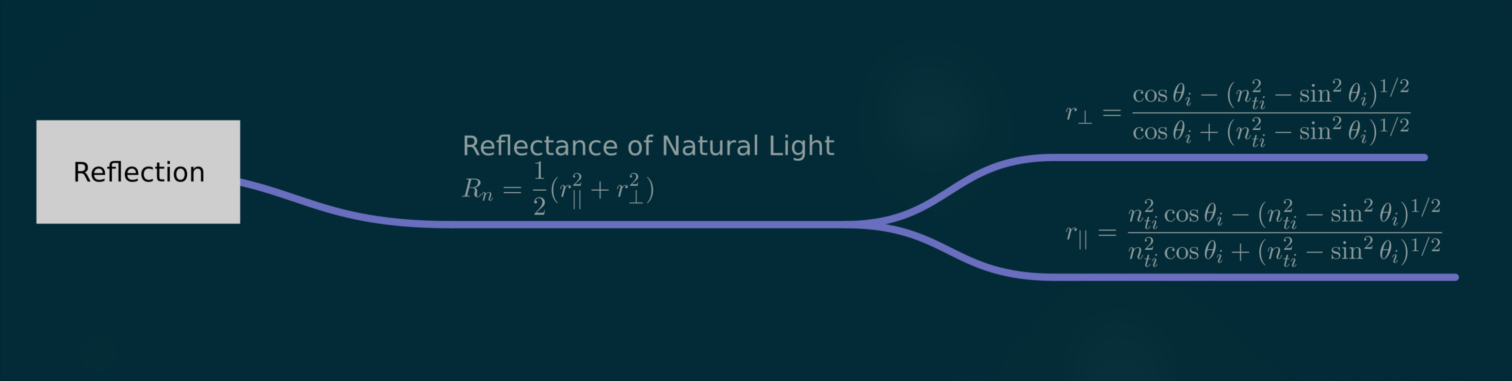
Original Reflection.png diagram. Click the image to view it at full size.

The index in the image is the relative index \(n_{ti}\), so the extra definitions are

\[n_{ti} = \frac{n_t}{n_i}, \qquad n_i=1, \qquad n_t=1.5.\]

With Y = R_n, X = theta_i, and Trig angles = Degrees, this plots reflectance from normal incidence to grazing incidence. Change \(n_t\) to provide the transmitted medium’s index; change \(n_i\) when the incident medium is not air. The dependency readout shows how the indices and angle produce the amplitude coefficients and then the reflectance. For equal indices the written formulas are singular at exactly \(90^\circ\); that endpoint is omitted rather than assigning a limit.

The supplied definition uses

\[R_n=\frac{1}{2}\left(|r_{\parallel}|^2+|r_{\perp}|^2\right).\]

For real amplitudes this agrees with the squares in the image. The modulus squares also give power reflectance when the amplitudes become complex, including total internal reflection. See the Fresnel equations reference. For the default indices, \(R_n(0)=0.04\). Setting \(n_i=1.5\) and \(n_t=1\) gives \(R_n=1\) above the critical angle of approximately \(41.81^\circ\). These are equations for a planar interface between transparent, homogeneous media; index inputs are real numbers.

The editor contains the entire calculation. You can use the exact r_{\parallel}^2 and r_{\perp}^2 expressions from the image instead; the evaluator follows what you entered and does not silently replace them with modulus squares.

Supported input

This is an evaluator for explicit scalar equations, rather than a solver for every possible mathematical statement. Each left side must be a single variable; for example, enter y = x^2 instead of f(x) = x^2.

Input	Examples
Variables and subscripts	x, R_n, n_{ti}, \theta_i, r_{\perp}, r_{\parallel}; use \mathrm{gain} for a multi-letter name. Bare ab means multiplication, not one name.
Arithmetic	+, -, *, \cdot, \times, /, \frac{a}{b}, x^2, x^{1/2}, 2x, \sqrt{x}, \sqrt[3]{x}, parentheses and braces.
Trigonometry	\sin, \cos, \tan, \cot, \sec, \csc, \arcsin, \arccos, \arctan, \sin^2 x. \sin^{-1}, \cos^{-1}, and \tan^{-1} mean inverse functions; write 1/\sin(x) for a reciprocal.
Exponentials and logarithms	\exp(x), e^x, \ln(x) (natural log), \log(x) (base 10), \log_{2}(x), \sinh, \cosh, \tanh.
Complex values	i is the imaginary unit. Intermediate values can be complex; |z| and \left|z\right| give their magnitude. Powers and roots use the principal complex branch.
Constants and formatting	\pi, e, and i are reserved. Math delimiters $...$, \[...\], and aligned/align wrappers are accepted, as are & alignment markers and \\ line breaks. % starts a comment to the end of the line.

Angle mode applies to every trigonometric function, and inverse trigonometric functions return values in the selected unit. Hyperbolic functions are unaffected. Changing angle mode does not convert the numbers in the editor or the X domain; change those bounds explicitly when needed. The plotter does not infer physical units or dimensional consistency.

Implicit or circular systems, derivatives, integrals, sums, matrices, piecewise definitions, and user-defined functions are not supported. They produce a diagnostic instead of an invented calculation. Duplicate definitions, syntax errors, and missing parameter values also prevent a plot from being shown.

Only finite real Y values are plotted. Undefined and non-real results leave gaps, with counts shown above the controls. The plot uses 501 uniformly spaced samples; narrow resonances or singularities between samples may be missed. Reduce the plotted interval to inspect rapid changes. This is not an adaptive sampler or a proof of continuity.

How the calculation is built

The browser parses LaTeX into an expression tree, checks the supported operations, and orders definitions so each dependency is evaluated before it is used. At each sampled X value, it inserts the parameter values and evaluates that ordered graph. The plotted result is determined by the equations, rather than a hard-coded reflection algorithm; the Gaussian example uses the same engine.

Parsing uses CortexJS LaTeX Syntax, and numerical complex arithmetic uses Complex.js. Both libraries are bundled with the documentation. Calculation and plotting run locally in the browser, without a Python kernel, external calculation service, or generated executable JavaScript. MathJax is only needed for the optional typeset preview. Inputs are not saved between page loads.