Pupil Sampling — A Lecture on Where the Rays Go

Every analysis in KrakenOS — spot diagrams, PSFs, MTF, OPD maps, Seidel sums, radiometric throughput, Monte-Carlo stray-light — ultimately estimates an integral over the entrance pupil:

\[I \;=\; \frac{1}{A}\int_{\text{pupil}} f\!\left(x_{\!p},\, y_{\!p}\right)\, dA \;\approx\; \frac{1}{N}\sum_{i=1}^{N} f\!\left(x_i,\, y_i\right)\]

Choosing the sample positions \(\{(x_i, y_i)\}\) is pupil sampling. The choice controls three different things at once: how fast the estimate converges, how isotropic the result is, and how much aliasing leaks into image-plane FFTs. This page surveys the strategies KrakenOS ships, derives the equal-area trick they all share, and motivates the Vogel / golden-angle spiral that the UI uses internally for source previews and Lambertian / lobe scattering.

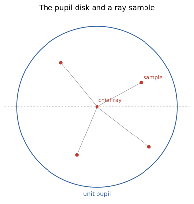
Unit pupil disk with a chief ray and a few sample points — The unit pupil \(\{(x_p, y_p) : x_p^2 + y_p^2 \le 1\}\). The chief ray sits at the centre; analysis rays are deposited on the disk and then mapped to real-world starting positions and direction cosines by `PupilCalc.Pattern2Field`.

1. What makes a sampler “good”?

Three useful quality metrics, all easy to read off the figures further down:

Equal area. Every sample should represent the same area of the pupil. If samples cluster near the centre, the Monte-Carlo estimate becomes a biased estimate of an axially-symmetric integrand. The fix is the radial mapping \(r = \sqrt{u}\) for \(u \in [0,1]\) derived below.
Low discrepancy. Loosely: no large empty regions and no clumps. Quantitatively, the star discrepancy \(D^*_N\) measures the worst-case deviation between sample density and true area. Truly random points have \(D^*_N \sim N^{-1/2}\); quasi-random sequences (Halton, Sobol, golden-angle) can reach \(D^*_N \sim N^{-1} \log^{d-1} N\).
Isotropy. Section fans deliberately collapse the pupil to a line and are fine for tangential / sagittal aberration plots. For PSFs, MTFs, and stray light you want sampling that does not pick a direction.

A useful empirical proxy for the last two is the nearest-neighbour distance distribution: a tight peak ≈ uniform spacing; a long left tail ≈ clumps.

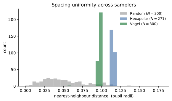
Nearest-neighbour distance histograms for random, hexapolar and Vogel — Nearest-neighbour distances for the three full-disk samplers at \(N \approx 300\). Random sampling produces clumps (left tail of short distances); hexapolar and Vogel are tightly peaked, with Vogel slightly narrower than hexapolar.

2. The equal-area mapping 

A common rookie mistake: place \(N\) samples by stepping \(r = i/N\) and rotating around. Because \(dA = r\, dr\, d\theta\), that recipe oversamples the centre by a factor of \(r\).

The fix follows from the inverse-CDF method. For uniform sampling on a disk of radius \(R\), the radial CDF is

\[F_R(r) \;=\; \frac{\pi r^{2}}{\pi R^{2}} \;=\; \frac{r^{2}}{R^{2}}, \qquad r \in [0, R].\]

Inverting \(F_R(r) = u\) with \(u \sim \mathcal{U}(0, 1)\) gives

\[\boxed{\;r \;=\; R \sqrt{u}\;}\]

so every linear, equal-spaced sequence in \(u\) produces an equal-area sequence in \(r\). This single identity is why KrakenOS’s Vogel sampler uses r = sqrt(i/N) and why the Random-disk generator works by rejection sampling on the unit square (which is equivalent to taking \(u \sim \mathcal{U}(0,1)\)).

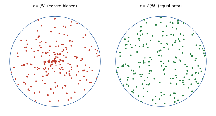
Centre-biased r = i/N versus equal-area r = sqrt(i/N) — Same 200 indices, two radial maps: \(r = i/N\) (left) over-densifies the centre, \(r = \sqrt{i/N}\) (right) gives constant area density.

3. Section fans — when one dimension is enough 

For tangential / sagittal aberration slices, a 2D sampler is wasteful: the integrand is constant along the orthogonal direction. KrakenOS exposes three section patterns (see Pupil Patterns (Source Model: Pupil / field)):

Fan Y (Pup.Ptype = "fany") — the meridional fan, \(\{(0, j/\mathrm{Samp})\}\). Canonical input for transverse ray-aberration plots \(\Delta y' = \mathrm{TRA}_y(p_y)\).
Fan X ("fanx") — sagittal fan.
Cross fan ("fan") — Fan X ∪ Fan Y, useful for a quick visual sanity check of both aberration directions in one trace.

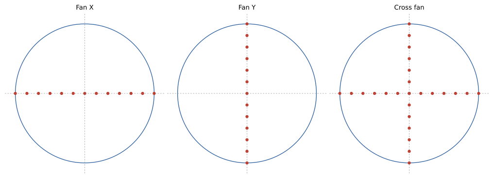
Fan X, Fan Y, and Cross fan patterns on the unit pupil — Section patterns. They are not physical 3D launch distributions; Open 3D source-cone tracing maps them to a filled angular cone.

Section fans converge as \(O(1/N^{2})\) for the 1D integrals they target (Simpson-like behaviour with smooth integrands) but they are not valid for any quantity that requires a 2D integral over the pupil — PSF, encircled energy, MTF, throughput.

4. Hexapolar — equal-area rings 

The traditional analysis default. One chief ray at the centre plus Samp concentric rings, ring \(j\) carrying \(6j\) samples evenly spaced in azimuth at radius \(r_j = j/\mathrm{Samp}\). Each ring covers an area \(\pi (r_j^2 - r_{j-1}^2) = \pi (2j-1)/\mathrm{Samp}^{2}\), and there are \(6j\) samples on it, giving constant per-sample area \(\pi (2j-1) / (6j\,\mathrm{Samp}^{2}) \approx \pi/(3\,\mathrm{Samp}^{2})\) for large \(j\) — so the pattern is asymptotically equal-area without the \(\sqrt{\cdot}\) step.

The total ray count is

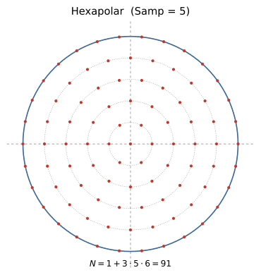
\[N_{\text{hex}} \;=\; 1 + \sum_{j=1}^{\mathrm{Samp}} 6j \;=\; 1 + 3\,\mathrm{Samp}(\mathrm{Samp}+1).\]

Hexapolar sampling with Samp = 5 — Hexapolar at `Samp = 5`: six-fold azimuthal symmetry and well defined ring radii. Deterministic, reproducible, and visually readable in spot diagrams.

Strengths: zero variance for any radially-symmetric integrand at finite \(N\); exact six-fold symmetry plays nicely with PSF cores. Weakness: the strong angular ordering aliases sharp pupil features (a hard mask, a vignette edge) into Moiré-like artefacts in FFTs.

5. Square grid — when the detector decides 

A Cartesian grid of step \(1/\mathrm{Samp}\) clipped to the unit disk (Pup.Ptype = "square"). It contains roughly \(\pi \mathrm{Samp}^{2}\) samples after clipping. Useful when:

The downstream computation is an FFT-based OPD → PSF pipeline that wants a square footprint anyway.
Sample positions must align with detector pixel centres in image space (e.g. discrete-grid optical-bench experiments).

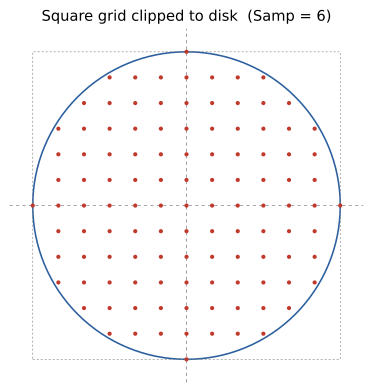
Square grid clipped to the unit disk — The Cartesian grid that survives the disk clip. The corner samples are dropped, leaving a slightly noisy boundary.

Weakness: the boundary is irregular, so a marginal-ray sweep produced by this pattern has gaps. Avoid for Seidel sums or marginal-rim analyses; prefer hexapolar or Vogel there.

6. Random disk — the Monte-Carlo baseline 

Pup.Ptype = "rand": rejection sampling on the square \([-1, 1]^2\) keeping points with \(x^2 + y^2 < 1\). Up to \(4\,\mathrm{Samp}^{2}\) candidates produce a disk population of roughly \(\pi \mathrm{Samp}^{2}\).

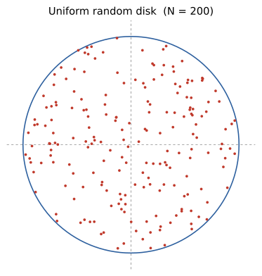
Uniform random samples on the disk — Uniform pseudo-random samples. Note the visible clumps and voids typical of low-\(N\) random draws.

For an integrand \(f\) with finite variance \(\sigma^{2}\), the standard Monte-Carlo error is

\[\operatorname{Var}\!\left[\hat{I}_{N}\right] \;=\; \frac{\sigma^{2}}{N}, \qquad \operatorname{StdErr} \;=\; \frac{\sigma}{\sqrt{N}}.\]

Strength: the rate \(1/\sqrt{N}\) is independent of dimension, which is why it remains the workhorse for high-dimensional stray-light integrals. Weakness: clumps and voids at small \(N\) produce visible banding in PSF / spot estimates.

7. The Vogel / golden-angle spiral 

This is the sampler KrakenOS uses inside the source preview, the reference-disk launcher, and the Lambertian / cosine-lobe hemisphere generators — see sample_source_disk_points in KrakenOS/UI/source_trace_helpers.py, the matching 3D variant sample_reference_disk_points_3d, and the hemisphere code in KrakenOS/KrakenSys.py. It is colloquially called “Fibonacci sampling” because its azimuthal step is the limit of the Fibonacci ratios.

Definition

For sample index \(i = 0, 1, \dots, N-1\):

\[r_{i} \;=\; R\sqrt{i / (N-1)}, \qquad \theta_{i} \;=\; i \cdot \alpha, \qquad \alpha \;=\; \pi\bigl(3 - \sqrt{5}\bigr) \;\approx\; 137.5077640^{\circ}.\]

The radial step is the equal-area mapping of §2. The azimuthal step \(\alpha\) is the golden angle.

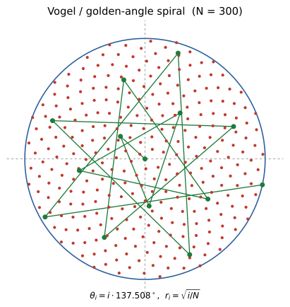
Vogel spiral with N = 300 points; the first 14 highlighted — \(N = 300\) Vogel samples. The green polyline highlights the first 14 in order — they spiral outward at exactly \(137.5^\circ\) per step.

Why the golden angle?

The golden angle is the unique angle that is maximally irrational in a number-theoretic sense, and that is what makes the resulting spiral low-discrepancy. The derivation has three steps.

Step 1 — turn fraction. Set \(\alpha = 2\pi\,\rho\) for some turn fraction \(\rho \in (0, 1)\). After \(N\) steps the azimuths are \(\{2\pi\,\rho\,i \bmod 2\pi\}\). If \(\rho = p/q\) is rational with small \(q\), every \(q^{\text{th}}\) sample lands on the same ray and you get \(q\)-arm starburst patterns instead of a uniform fill.

Step 2 — continued fractions. The “how rational” of any \(\rho\) is measured by how well it can be approximated by rationals. Every irrational \(\rho\) has a unique simple continued-fraction expansion \(\rho = [a_{0}; a_{1}, a_{2}, \dots]\). Large \(a_{k}\) mean cheap rational approximations (close clumps); small \(a_{k}\) mean the opposite. The most-irrational choice is the one where every \(a_{k} = 1\):

\[\rho^{*} \;=\; [0; 1, 1, 1, 1, \dots] \;=\; \frac{1}{1 + \dfrac{1}{1 + \dfrac{1}{1 + \dotsb}}} \;=\; \frac{1}{\varphi}, \quad \varphi = \frac{1+\sqrt{5}}{2}.\]

Step 3 — back to the angle. Either turn fraction \(\rho^{*}\) or \(1 - \rho^{*}\) works; by convention we take

\[\alpha \;=\; 2\pi\bigl(1 - 1/\varphi\bigr) \;=\; \frac{2\pi}{\varphi^{2}} \;=\; \pi(3 - \sqrt{5}) \;\approx\; 137.5078^{\circ}.\]

The successive Fibonacci ratios \(F_{n}/F_{n+1} = 1/1, 1/2, 2/3, 3/5, 5/8, 8/13, \dots\) are exactly the convergents of the continued-fraction expansion, which is why this angle is also called the Fibonacci angle even though no Fibonacci number appears in the runtime formula.

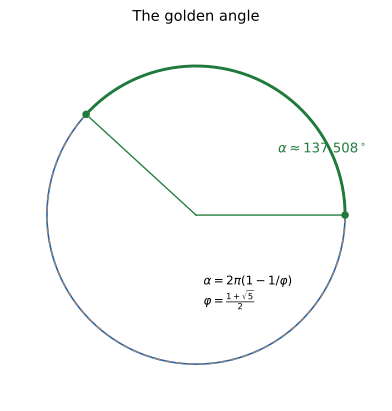
The golden angle on the unit circle — The golden angle as a fraction of the full circle. The green arc is the turn taken between successive samples; the grey-dashed arc is the *complement* taken on every other revolution. Neither arc closes into a low-period orbit.

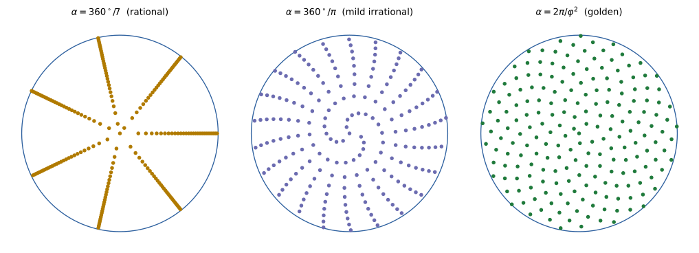
Spirals at three different turn angles — Same \(N = 200\) indices, three angles. A *rational* angle (\(360^{\circ}/7\)) produces seven straight arms. A *mildly irrational* angle (\(360^{\circ}/\pi\)) still shows visible curved bands. The **golden angle** uniformly fills the disk.

Why optical designers care

Convergence. For smooth integrands the Vogel spiral behaves like a 2D quasi-random sequence: error \(\sim N^{-1}\) versus \(N^{-1/2}\) for pure random. In a typical PSF estimate you reach the same standard error with \(\sim \sqrt{N_{\text{random}}}\) rays.
Isotropy. Unlike the hexapolar grid, the Vogel spiral has no preferred direction at any \(N\), so it never imprints six-fold structure on a PSF or MTF.
Incremental. Adding samples never re-positions existing ones. This makes it ideal for live UI previews: increase ray_count and the previously drawn rays remain valid — a property the sample_source_disk_points helper relies on.
Boundary fill. The outermost ring is exactly \(r_{N-1} = R\), so the marginal rim is always sampled. The square-grid and random-disk patterns leave a fluctuating gap there.

8. From disk to hemisphere — Lambertian and lobe scattering 

The same spiral lifts straight onto a hemisphere. KrakenOS’s Lambertian emitter (KrakenSys.py around line 2565) and its glossy lobe (line 2602) both use it.

For a cosine-weighted hemisphere (Lambert’s law), the joint PDF in spherical coordinates is \(p(\theta, \phi) = \cos\theta\,\sin\theta / \pi\). Integrating gives the marginal radial CDF

\[F(\theta) \;=\; \sin^{2}\theta, \qquad F^{-1}(u) \;=\; \arcsin \sqrt{u},\]

so the recipe is

\[\sin^{2}\theta_{i} \;=\; i/N, \qquad \phi_{i} \;=\; i\cdot \alpha,\]

which is exactly what KrakenSys._sample_lambertian_directions does (sin2_max clamps the cone). The Vogel spiral on the disk maps isomorphically onto the cosine-weighted hemisphere by reading the disk-radius \(r_{i} = \sqrt{i/N}\) as \(\sin\theta_{i}\).

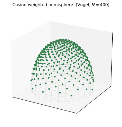
Vogel samples lifted onto a cosine-weighted hemisphere — 400 directions drawn from the cosine-weighted hemisphere using the Vogel spiral with \(\sin^{2}\theta = i/N\). The density falls off toward the rim because Lambert’s law puts more flux near the normal.

The directional-lobe variant raises the cosine to a power \(n\) (settings["lobe_exponent"]), giving a glossy specular highlight; the golden-angle azimuth keeps the lobe rotationally uniform.

9. KrakenOS code map 

Where each sampler lives, for reference:

KrakenOS sampling sites
Sampler	Where it is implemented	Where it is used
Hexapolar / Square / Random / fans	`KrakenOS/PupilTool.py` (`PupilCalc.Pattern`)	Sequential analysis driven by `Pup.Ptype`; UI labels in `PUPIL_PATTERN_TO_KRAKEN`.
Vogel disk (2D)	`sample_source_disk_points` — `KrakenOS/UI/source_trace_helpers.py`	2D source previews; non-sequential disk launches with `ray_count > 9`.
Vogel disk (3D)	`sample_reference_disk_points_3d` — same file	Open 3D scene reference launches.
Vogel preview overlays	`KrakenOS/UI/services/source_modeling.py` and `KrakenOS/UI/services/trace_preview_sampling.py`	Live “Source preview” and “Trace preview” overlays in the Layout Editor.
Vogel hemisphere (Lambertian)	`KrakenSys.py` `_sample_lambertian_directions`	Diffuse scattering from a surface; non-sequential thermal / Lambertian sources.
Vogel cosine-lobe	`KrakenSys.py` directional-lobe block	Glossy specular scattering with adjustable `lobe_exponent`.
Vogel finite-source offsets	`KrakenSys.py` finite-source pupil block	Mapping a finite-radius emitter to a Lambertian fan when `Source cone` is non-zero.

10. Choosing in practice 

A short decision tree for the analyses the Layout Editor surfaces:

Tangential aberration plot, sagittal aberration plot, ray-fan display — Fan Y or Fan X (then maybe Cross fan).
Spot diagram, Seidel sums, ABCD/wavefront overlay, classical OPD — Hexapolar at Samp = 5…8 (deterministic, six-fold benign).
Square-detector PSF / FFT-OPD pipeline — Square grid; align Samp to the detector sampling.
Encircled energy, throughput, stray-light Monte-Carlo, edge-of-pupil vignetting — Vogel (via source preview / disk launchers) or Random if you need an unbiased variance estimate.
Non-sequential diffuse / glossy surface scattering — leave it to the built-in Lambertian and lobe samplers, both of which already use the golden-angle spiral.

When in doubt: start with hexapolar for analysis and Vogel for source launches. They cover almost every workflow in KrakenOS.