Folded Coaxial Illumination — Projection Physics and the MV-150

A flat mirror or beam splitter changes a ray bundle’s direction; it does not, by itself, magnify one transverse axis. The familiar \(\cos\theta\) factor belongs to the projection of a finite aperture whose size is measured in the tilted plane. It must not be applied a second time to a cube side that is already the aperture’s projected width.

There is a second distinction which matters just as much: a 30 mm collimated beam and a 30 mm Lambertian emitter are not the same thing. The former has a defined cross-section; the latter has both a spatial extent and a distribution of ray angles.

This page develops the general construction first, illustrates four common under-fill and over-fill cases, and then applies it to the MV-150 layout’s 55 × 55 × 78 mm beam-splitter solid. It also records the actual MV-150 experiment: a 55 × 74 mm flat LED with diffuser produces two side dark edges and an approximately 35 × 39 mm usable bright region inside the 39 × 39 mm FOV.

Keep these five quantities separate

Quantity	Meaning
Emitter size	The physical luminous area. It does not define a unique beam width unless the angular distribution and any relay optics are also known.
Beam cross-section	The bundle shape measured in a plane normal to its chief ray.
Splitter footprint	The intersection of that bundle with the tilted splitter plane. It is longer than the normal beam section along the plane of incidence.
Clear aperture	The usable optical opening after coating borders, bevels, mounts and windows are included. Mechanical outside dimensions are only an upper bound.
Illuminated object field	The irradiance distribution on the Object plane after propagation, clipping, refraction and radiometric weighting.

Most incorrect \(\cos45^\circ\) arguments come from substituting one row of this table for another.

General rule for an ideal planar fold

For a unit splitter normal \(\mathbf n\), specular reflection maps an incident direction \(\mathbf d\) to

\[\mathbf d_{\mathrm r} = \mathbf d - 2(\mathbf d\!\cdot\!\mathbf n)\mathbf n .\]

Derivation by normal and tangential components

Assume \(\mathbf d\) and \(\mathbf n\) are unit vectors, and let \(\mathbf d\) point in the direction of travel toward the splitter. The vector projection of \(\mathbf d\) onto the surface normal is

\[\mathbf d_\perp = \operatorname{proj}_{\mathbf n}(\mathbf d) = (\mathbf d\!\cdot\!\mathbf n)\mathbf n .\]

Subtracting that projection leaves the component parallel to the splitter:

\[\mathbf d_\parallel = \mathbf d-\mathbf d_\perp = \mathbf d-(\mathbf d\!\cdot\!\mathbf n)\mathbf n .\]

Ideal specular reflection keeps the tangential component and reverses only the normal component. Therefore

\[\begin{split}\begin{aligned} \mathbf d_{\mathrm r} &= \mathbf d_\parallel-\mathbf d_\perp \\ &= \left[\mathbf d-(\mathbf d\!\cdot\!\mathbf n)\mathbf n\right] -(\mathbf d\!\cdot\!\mathbf n)\mathbf n \\ &= \boxed{\mathbf d-2(\mathbf d\!\cdot\!\mathbf n)\mathbf n}. \end{aligned}\end{split}\]

Geometrically, subtracting \(\mathbf d_\perp\) once brings the vector head onto the tangent plane; subtracting the same component a second time moves it an equal distance to the reflected side. That is the origin of the factor 2—it is not a beam-width scale factor.

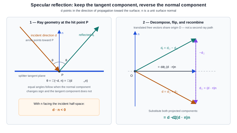
With the normal drawn toward the incident half-space, \(\mathbf d\!\cdot\!\mathbf n<0\); hence \(\mathbf d_\perp\) points into the surface. Reflection changes it to \(-\mathbf d_\perp\), while \(\mathbf d_\parallel\) is unchanged. The two vector additions in the right panel reconstruct \(\mathbf d\) and \(\mathbf d_{\mathrm r}\).

The result satisfies the reflection law directly. Its normal component has equal magnitude and opposite sign,

\[\mathbf d_{\mathrm r}\!\cdot\!\mathbf n = -\mathbf d\!\cdot\!\mathbf n,\]

while its tangential component is unchanged. Because the two components are orthogonal,

\[\lVert\mathbf d_{\mathrm r}\rVert =\lVert\mathbf d\rVert=1.\]

For a normal facing the incident half-space, the directed-vector statement of equal incidence and reflection angles is

\[\angle(-\mathbf d,\mathbf n) =\angle(\mathbf d_{\mathrm r},\mathbf n).\]

Thus the physical incident and reflected ray lines obey equal angles even though \(\mathbf d\) itself points toward the hit point. Reversing the chosen normal (\(\mathbf n\rightarrow-\mathbf n\)) leaves the formula unchanged. If a non-unit normal is supplied, use

\[\mathbf d_{\mathrm r} = \mathbf d -2\frac{\mathbf d\!\cdot\!\mathbf n} {\mathbf n\!\cdot\!\mathbf n}\mathbf n .\]

This is an orthogonal transformation: it preserves distances and angles. Consequently, an unclipped collimated square remains congruent to the square, and an unclipped circular bundle remains circular, when each is measured in a plane normal to its own chief ray.

The splitter-plane footprint is different. If \(W\) is a beam width normal to the incident chief ray and the splitter is at angle \(\theta\) to that transverse plane, then

\[W_{\mathrm{footprint}} = \frac{W}{|\cos\theta|}.\]

Conversely, if \(A\) is a clear length measured along the tilted splitter plane, its accepted transverse width is

\[C_{\mathrm{fold}} = A|\cos\theta|.\]

Here \(\theta\) is the surface tilt relative to the incident transverse plane—equivalently, the incidence angle from the surface normal. For a specular fold, the chief ray deviates from its original direction by \(\delta = 180^\circ - 2\theta\) — not \(2\theta\); at 45° both expressions give 90°, which is what lets that shorthand survive casual checks. Thus a 90° path turn uses \(\theta=45^\circ\); the KrakenOS field named coaxial_fold_angle_deg currently stores this 45° surface/incidence angle, not the 90° change in propagation direction.

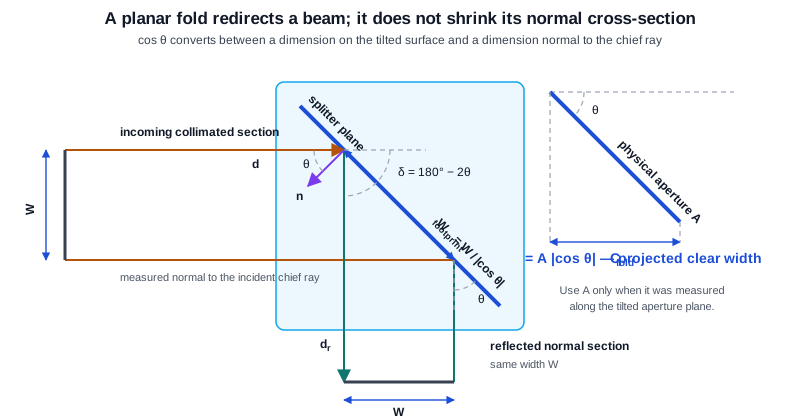
The reflection-law vectors are drawn at the upper hit point: incident direction \(\mathbf d\), surface normal \(\mathbf n\), reflected direction \(\mathbf d_{\mathrm r}\), the incidence angle \(\theta\) between \(-\mathbf d\) and \(\mathbf n\), and the deviation \(\delta = 180^\circ - 2\theta\) measured from the un-deflected continuation. The incoming and reflected normal sections both have width \(W\); only the splitter footprint is \(W_{\mathrm{footprint}} = W/|\cos\theta|\). The inverse calculation, \(C_{\mathrm{fold}} = A|\cos\theta|\), converts a physical tilted-aperture length \(A\) back to accepted normal beam width.

For a rectangular collimated bundle with incident widths \(W_f\times W_p\) and a projected clear aperture \(C_f\times C_p\),

\[W_{f,\mathrm{out}}=\min(W_f,C_f), \qquad W_{p,\mathrm{out}}=\min(W_p,C_p).\]

The subscripts f and p mean fold axis and perpendicular axis. This minimum rule describes the support of centred, axis-aligned geometrical rays. It does not describe penumbra or irradiance.

Case 1 — underfilled square bundle

If \(W_f<C_f\) and \(W_p<C_p\), no ray is clipped. An ideal 30 × 30 mm collimated square therefore remains 30 × 30 mm after a 90° fold, apart from a rotation or mirror reversal of its coordinate labels.

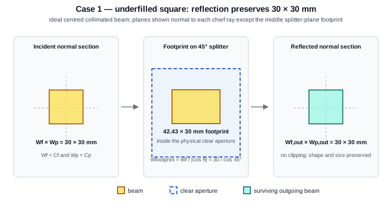
Reflection redirects the bundle but does not apply anamorphic magnification. This statement assumes collimation, an Object plane normal to the outgoing chief ray, and no other limiting stop.

Case 2 — underfilled circular bundle

If a circular bundle of diameter \(D\) fits inside the projected clear aperture, it remains a circle of diameter \(D\) after reflection.

Its footprint on the tilted splitter is an ellipse with axes \(D/|\cos\theta|\times D\). That ellipse is an intersection shape on the splitter surface, not the outgoing beam section.

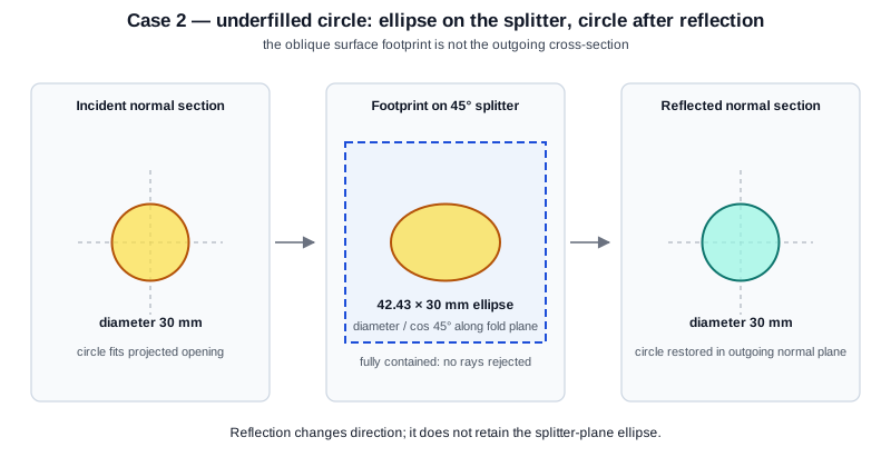
At 45°, a 30 mm circle occupies approximately 42.43 × 30 mm on the splitter plane. If that footprint fits, the reflected normal section is still a 30 mm circle.

Case 3 — overfilled square bundle

When a square or rectangular collimated bundle is larger than the projected clear aperture, the aperture clips it. For example, a 70 × 70 mm bundle and a 55 × 78 mm projected opening give

\[\min(70,55)\times\min(70,78)=55\times70\ \mathrm{mm}.\]

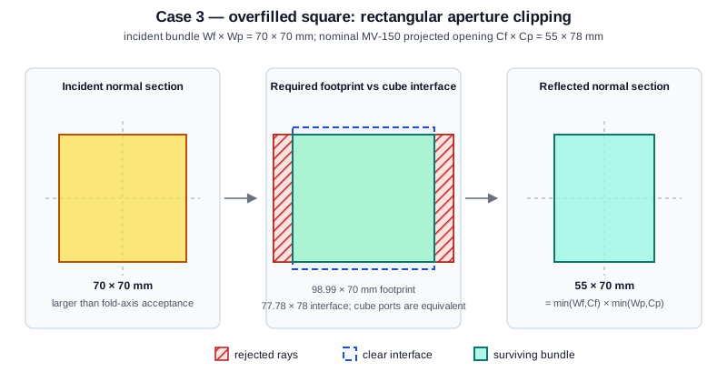
The rectangle is caused by clipping at a rectangular projected aperture. It is not a deformation imposed by specular reflection. In the actual cube the normal entry port and the projected diagonal have the same nominal 55 × 78 mm acceptance; the first encountered usable opening clips the rays.

Case 4 — overfilled circular bundle

A circle clipped by a rectangular aperture does not generally become an ellipse. Its outgoing support is

\[\Omega_{\mathrm{out}} = \left\{x^2+y^2\leq(D/2)^2\right\} \cap \left\{|x|\leq C_f/2,\ |y|\leq C_p/2\right\}.\]

For \(D=70\ \mathrm{mm}\) and \(C_f\times C_p=55\times78\ \mathrm{mm}\), the perpendicular 78 mm opening does not clip the circle, but the 55 mm fold-axis opening removes two circular segments. The result has a 55 × 70 mm bounding box and two flat sides.

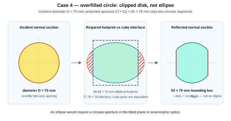
A true ellipse results when a circular aperture located in the tilted plane is projected onto a normal plane, or when an anamorphic optical system is present. It is not the generic result of clipping a circular beam with a rectangular cube opening. The middle panel compares the footprint that the unvignetted beam would require with the diagonal interface; a real normal-incidence cube port may clip it first.

External and internal reflection

The geometrical reflection law is the same for an external coated mirror, an internal coated interface and total internal reflection. What changes is the radiometry: Fresnel coefficients, polarization, phase, absorption and ghost paths.

A cube also has entry and exit refractions. In the centred MV-150 chief-ray geometry those faces are normal to the incoming and outgoing chief rays, so they do not introduce a universal fold-axis scale. Off-axis or divergent rays can acquire lateral shifts and different clipping, which is another reason to ray-trace a real area source instead of assigning a hard footprint from one nominal dimension.

The actual MV-150 beam-splitter geometry

The promoted MV-150 optical solid has bounds 55 mm in the fold-plane X direction, 55 mm in Z and 78 mm perpendicular to the fold. Its entry and exit face extents are therefore 55 × 78 mm. These CAD extents are a nominal geometric upper bound, not a measured usable clear aperture.

The internal 45° interface crosses the complete 55 × 55 mm square. Its physical length in the tilted plane is

\[A_{\mathrm{diagonal}} = \sqrt{55^2+55^2} = 55\sqrt2 = 77.7817\ \mathrm{mm}.\]

The CAD face area confirms this:

\[77.7817\times78 = 6066.976\ \mathrm{mm^2}.\]

Projecting the actual nominal diagonal extent gives

\[C_f = (55\sqrt2)\cos45^\circ = 55\ \mathrm{mm}, \qquad C_p=78\ \mathrm{mm}.\]

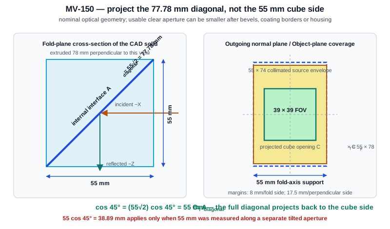
The \(\cos45^\circ\) projection is real, but its input is the 77.78 mm diagonal—not the already projected 55 mm cube side. Applying \(55\cos45^\circ\) a second time double-counts the projection. Bevel, coating-border, housing and window dimensions are still needed to turn this nominal acceptance into a true clear aperture.

For ideal centred collimated bundles, the nominal MV-150 results are:

Incident bundle	Output after the cube	Shape
30 × 30 mm square	30 × 30 mm	Unclipped square
30 mm diameter circle	30 mm diameter	Unclipped circle
70 × 70 mm square	55 × 70 mm	Rectangularly clipped
70 mm diameter circle	55 × 70 mm bounding box	Circle with two clipped sides
MV-150 55 × 74 mm collimated rectangle	55 × 74 mm	Fits the nominal 55 × 78 mm opening

Intersecting that last collimated support with the 39 × 39 mm object-space FOV gives a fully covered 39 × 39 mm field. The nominal cube dimensions alone therefore do not predict two dark edges.

A result of \(55\cos45^\circ=38.8909\ \mathrm{mm}\) would be correct only if 55 mm were independently measured along a separate tilted clear aperture. For example, a 55 mm plate-mirror opening at 45° would present 38.8909 mm to the beam. That is not the geometry of the full internal diagonal in this 55 mm cube.

Reported physical MV-150 camera result — approximately 35 × 39 mm bright

The user-reported physical MV-150 experiment used the 55 × 55 × 78 mm beam-splitter solid and a 55 × 74 mm flat LED with a diffuser. The recorded camera image, mapped to the 39 × 39 mm object-space FOV, shows two dark side edges. Taking those sides as the fold axis, the approximate usable-bright region is

\[35\ \mathrm{mm}\quad\text{(fold axis)} \;\times\; 39\ \mathrm{mm}\quad\text{(perpendicular axis)}.\]

For a centred pattern, the fold-axis shortfall is approximately

\[39-35=4\ \mathrm{mm}, \qquad \frac{4}{2}\approx2\ \mathrm{mm}\]

at each side. “Usable bright” is an image-intensity threshold or contour, not a hard geometrical support boundary. Its numerical width depends on the threshold, exposure, flat-field calibration and measurement uncertainty; those quantities have not yet been specified.

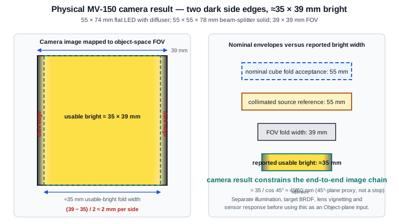
The reported end-to-end asymmetry is real: recorded camera intensity rolls off along the fold axis while the perpendicular direction remains usable. It constrains the complete illumination–object–imaging–sensor chain, not the illuminator or nominal cube diagonal in isolation.

This observation and the nominal projection calculation are not contradictory. The nominal full-face collimated model predicts geometric illumination support beyond the complete FOV; the experiment says the end-to-end recorded intensity falls below its usable-bright criterion near the two fold-axis edges. Therefore at least one non-ideal or unmodelled mechanism is load-bearing, for example:

• a smaller coating, illuminator window, bevel or housing clear aperture;

• diffuser angular distribution and source/aperture view factor;

• decentre, tilt, gap or assembly tolerance;

• splitter throughput versus incidence angle and polarization;

• Object-plane BRDF or downstream lens/pupil vignetting.

Under an ideal centred, collimated, single-aperture orthographic-projection model, if the 35 mm threshold contour were represented as an equivalent hard aperture lying in a 45° plane, its in-plane width would be

\[A_{\mathrm{equivalent}} = \frac{35}{\cos45^\circ} \approx49.50\ \mathrm{mm}.\]

This 49.50 mm value is only a fitted proxy inside that ideal model. It is not proof that a physical 49.50 mm stop exists. A diffuser normally produces a soft irradiance transition rather than a hard support boundary.

Use the reported camera profile as an end-to-end validation target. Feed it back as Object-plane illumination only after a flat diffuse target and flat-field calibration have separated illumination from target BRDF, imaging-lens relative illumination and sensor response; otherwise those factors would be counted twice. For illumination-only coupling, use a calibrated Object-plane irradiance map or a physical source trace. Describe 35 × 39 mm as an approximate usable-bright threshold contour or width—not as the ray bundle’s hard support.

What the latest full KrakenOS recording shows—and does not show

The latest full UI recording, attachment/recorded_bug_repros/recording_20260719_095137.json, contains one flag: “All other Analysis Overlay no longer working, only the Illumination Overlay is working now.” It is a recording of the simulated 3D detector relative-illumination overlay, not a recording of the physical camera experiment. Its overlay qualitatively has the same two-side orientation—dark left and right edges, without comparable top and bottom edges.

For that simulation, the scene source is enabled as a 55 × 74 mm cosine-weighted/Lambertian emitter, but the current imaging-launch descriptor still constructs a synthetic fold-axis width \(55\cos45^\circ=38.8909\ \mathrm{mm}\). The visual map additionally uses a default raised-cosine penumbra of 6% of that width—approximately 2.33 mm—and Gaussian display smoothing with a 1.5-bin sigma. Consequently, any numerical bright width inferred by thresholding the screenshot depends on software heuristics and the chosen threshold. The visual resemblance to the reported approximately 35 × 39 mm physical result is useful for comparison, but it is not independent validation of that result or of the \(55\cos45^\circ\) interpretation.

The MV-150 source is Lambertian, not collimated

The saved MV-150 source is a 55 × 74 mm cosine-weighted emitter with a 90° cone. Each source point emits a hemisphere of directions. A plane splitter creates a same-size virtual source, but it does not form a 1:1 real image of that source on the Object plane.

Unfolding the reflection turns the path into ordinary free-space propagation. For a finite cone of half-angle \(\alpha\) and unfolded distance \(L\), the geometrical support is approximately the source shape expanded by \(L\tan\alpha\) on every side:

\[\Omega_{\mathrm{object}} \approx \Omega_{\mathrm{source}} \oplus \operatorname{disk}(L\tan\alpha).\]

A full Lambertian hemisphere has no finite hard support without apertures. Its irradiance falls with angle and distance, while the cube, housing, windows and other stops bound the visible source solid angle.

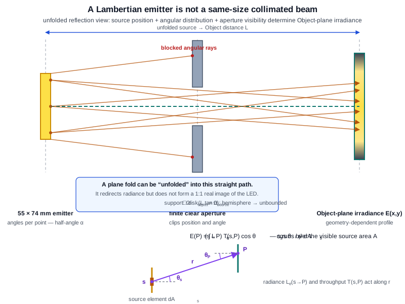
A physical emitter size is not a beam cross-section. The object receives an irradiance distribution assembled from all source points and all accepted directions, propagated in straight lines over the unfolded distance \(L\). The lower band draws the irradiance-integral geometry: a source element \(\mathrm dA_s\) around \(s\), the object point \(P\), their separation \(r\), and the obliquity angles \(\theta_s\) and \(\theta_P\) to the two plane normals.

At an Object-plane point \(P\), a useful radiometric statement is

\[E(P) = \int_{A_{\mathrm{visible}}} L_e(s\rightarrow P)\, T(s,P)\, \frac{\cos\theta_s\cos\theta_P}{r^2} \,\mathrm dA_s ,\]

where \(T\) includes aperture visibility, splitter throughput, refraction and losses. For a diffuse Object plane, this irradiance map and the surface reflectance/BRDF determine the radiance launched toward the camera. For a specular Object plane, the directional incident radiance \(L(x,y,\boldsymbol\omega)\) and the BRDF must be retained; a scalar irradiance map alone is insufficient. The integral is written in the unfolded/virtual-source geometry: \(r\) is the unfolded distance from source point \(s\) to \(P\), \(\theta_s\) and \(\theta_P\) are angles to the corresponding plane normals, and \(A_{\mathrm{visible}}\) is the source area visible through all projected stops.

How to predict dark edges generally

Use the following sequence for any folded illuminator:

1. Identify whether each quoted dimension describes an emitter, a collimated beam, a mechanical body or an optical clear aperture.

2. Express every clear aperture in a plane normal to the local chief ray. Use \(A|\cos\theta|\) only when \(A\) was measured along a tilted plane.

3. For a collimated bundle, intersect its transverse support with all projected apertures. For a divergent or Lambertian source, trace or integrate the accepted angular distribution.

4. Compute the object-plane irradiance \(E(x,y)\) over the complete imaged FOV.

5. Convey the illumination to the imaging calculation as ray weights or an illumination map for a diffuse object, or as directional radiance for a specular object. Cropping Object-plane launch coordinates is appropriate only for genuinely zero illumination outside a hard boundary.

6. Predict two dark edges only when irradiance rolls off inside the FOV on one axis while remaining flat on the perpendicular axis.

Possible physical causes include a smaller illuminator window, coating clear aperture, bevel or mount; source-view-factor roll-off; decentre; and downstream vignetting. They must be measured or modelled rather than inferred from the nominal 55 mm cube side.

KrakenOS descriptor semantics and the legacy MV-150 approximation

KrakenOS currently evaluates the coaxial descriptor as

\[C_f = \mathtt{coaxial\_aperture\_fold\_mm} |\cos(\mathtt{coaxial\_fold\_angle\_deg})| .\]

That formula is physically meaningful only if coaxial_aperture_fold_mm is an in-plane tilted-aperture length. The following block shows how the existing formula would encode the nominal full MV-150 diagonal:

{
    "coaxial_illuminator": True,
    "coaxial_aperture_fold_mm": 77.78174593,  # 55*sqrt(2), on diagonal
    "coaxial_aperture_perp_mm": 78.0,
    "coaxial_fold_angle_deg": 45.0,
    "coaxial_fold_axis": "x",
}

This evaluates to the cube’s nominal 55 × 78 mm transverse acceptance. It is not a complete physical MV-150 descriptor: the current schema carries one rectangle and does not independently represent and intersect the 55 × 74 mm source support, the cube acceptance, other clear apertures and the FOV. That separation requires either a richer schema or the physical trace. In this particular example both the nominal source and cube envelope over-fill the 39 × 39 mm FOV, so the missing distinction does not change the ideal collimated coverage verdict.

Warning

The existing MV-150 prescription supplies 55 mm together with 45°. The current kernel consequently constructs a synthetic 38.8909 mm fold-axis bound and can force two dark edges. That is a legacy approximation, not a result derived from the prescription’s 55 × 55 × 78 mm CAD solid. Its implementation guards demonstrate current software behaviour; they are not evidence for the physical projection. The synthetic 38.8909 mm support and the user-reported physical 35 mm usable-bright threshold width are different quantities and must not be presented as the same measurement.

For the actual Lambertian source, the preferred general solution is to trace the source through the true optical clear apertures. Accumulate \(E(x,y)\) for a diffuse Object plane, or retain directional radiance for a specular one, and carry the resulting weights through the imaging rays to the detector-relative-illumination overlay.