Chapter 16: Direct Modulation of Semiconductor Lasers
Source: Hunsperger, sixth edition (2009), Problems 16.1–16.9, printed pages 340–342. Static transfer-curve sketches neglect carrier dynamics unless explicitly included.
Problem 16.1 — Sinusoidal drive above the knee
Working. A 200 mA peak-to-peak signal has amplitude 100 mA: \(I(t)=300+100\sin\Omega t\) mA. The source graph has a knee near 200 mA, so the drive runs from that knee to approximately 400 mA. Along the nearly linear upper branch,
Answer. Draw an approximately sinusoidal optical output between the powers read at 200 and 400 mA, approximately 0.4–6 mW at the graph’s precision.
Check. At the trough the device is near the nonlinear knee, so exact linearity requires a little more DC bias.
Problem 16.2 — Drive crossing threshold
Working. Now \(I(t)=150+100\sin\Omega t\) mA, ranging from 50 to 250 mA. The stimulated-emission branch is reached only when \(\sin\Omega t>0.5\). A thresholded model is \(P_{\rm stim}\propto\max(0,I-200\,{\rm mA})\).
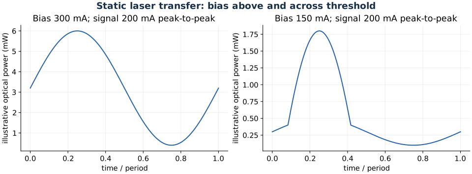
Static illustrative transfer curves with the source graph’s approximate knee.
Answer. Draw clipped optical peaks occupying about one third of the cycle, riding on a weak spontaneous-emission background.
Check. The electrical current never becomes negative. Clipping is caused by crossing the lasing knee, not by current reversal.
Problem 16.3 — Minimum DC bias for undistorted modulation
Working. Infer \(\Delta\nu=1.48119\times10^{13}\) Hz from 880 and 920 nm. For a confined-field DH laser, take \(D=d=1\,\mu{\rm m}\). With \(n=3.3,\eta_q=0.8\), \(L=0.1\) cm, and \(R=0.4\), (1) gives \(J_{\rm th}=192.077\,{\rm A/cm^2}\). The injection area is \(10^{-3}\,{\rm cm^2}\).
Answer. Slightly above 242 mA supplies margin over the ideal lower limit.
Check. Use half the 100 mA peak-to-peak signal as amplitude. If optical confinement is less than unity, the required bias is larger.
Problem 16.4 — Maximum linear modulation depth with a finite pedestal
Working. Avoiding below-threshold clipping limits sinusoidal current amplitude to \(130-100=30\) mA. The upper-branch slope in normalized optical power is \(S=(1-0.05)P_p/(300-100)\,{\rm mA}\). Therefore
Answer. Maximum undistorted modulation index is \(\delta P/P_{\rm dc}=0.74026\), about 74.0 percent.
Check. The current at the positive peak is only 160 mA, below the quoted 300 mA reference. If clipping and switching below threshold are permitted, this is no longer the relevant linear-modulation bound.
Problem 16.5 — Zero-bias turn-on delay and duty cycle
Working. For an initially empty carrier reservoir, the simple rate equation gives
Duty cycle alone would bound a 0.8 ns electrical pulse train by \(f\le0.05/(0.8\,{\rm ns})=62.5\) MHz. But such a first electrical pulse ends before the calculated turn-on delay.
Answer. Carrier buildup, pulse duration/duty cycle, and relaxation dynamics all constrain operation. If 0.8 ns denotes the desired optical pulse, the drive must last approximately \(0.8+0.863=1.663\) ns, giving an illustrative duty-limited bound of about 30.1 MHz. If it denotes electrical pulse width, the stated zero-initial-carrier model does not produce that first laser pulse.
Check. The interpretation of pulse width matters. Residual carriers in a repeating train require a periodic rate-equation calculation rather than repeatedly assuming zero initial population.
Problem 16.6 — Mechanisms limiting direct modulation
Working. Carrier and photon populations respond through coupled rate equations, producing relaxation oscillations and damping. Injection and transport take finite time. Junction capacitance, series resistance, contacts, and package inductance restrict the electrical drive. Thermal changes are slower still.
Answer. The useful bandwidth is bounded by both intrinsic carrier-photon dynamics and extrinsic electrical/transport response.
Check. Carrier lifetime by itself is not always the bandwidth limit above threshold: stimulated emission changes the dynamical response. Evaluate the small-signal transfer function at the operating bias.
Problem 16.7 — A route to fifty-gigahertz modulation
Working. In the textbook’s design context, ordinary direct-current modulation encounters relaxation, parasitic, and chirp limits at microwave frequencies. Keep a laser operating continuously and pass its beam through a separate fast electro-optic modulator. A traveling-wave electrode can match electrical and optical propagation and reduce lumped-capacitance limitations.
Answer. A traveling-wave Mach–Zehnder or suitable external electroabsorption modulator is a possible architecture for the 50 GHz design target.
Check. Ten gigahertz is not a universal physical ceiling for every semiconductor laser. The exercise describes a technology/design constraint, not a theorem independent of device structure.
Problem 16.8 — Delay of the first remote-sensor pulse
Working. For zero initial carriers, use \(\tau_s=300\) ns, \(I_p=5\) mA, and \(I_{\rm th}=1\) mA:
Answer. Approximately 66.9 ns before first threshold crossing.
Check. This excludes optical propagation time and receiver delay. Keeping a subthreshold bias would reduce carrier buildup time at the cost of standby power.
Problem 16.9 — Two-cavity Vernier spacing
Working. The optical lengths are \(n_1L_1=1035\,\mu{\rm m}\) and \(n_2L_2=1110.4\,\mu{\rm m}\). Using the usual weak-dispersion Vernier-envelope approximation,
Answer. Approximately 1.988 THz between envelope alignments, equivalent locally to about 5.99 nm near 950 nm.
Check. This is not a full calculation of adjacent coupled-cavity supermode splitting. That requires coupling and boundary conditions; group indices replace phase indices when dispersion matters.