Active Fiber Alignment: Power, Dither, and Spatial Sensing

Active alignment adjusts the relative position and angle of a beam and a fiber to maximize useful guided power. A practical starting point is a calibrated power measurement, a bounded search to find first light, and small controlled perturbations to optimize coupling. Cameras can accelerate acquisition when they observe the incident beam relative to the fiber.

The central design question is which measurement contains a repeatable, signed signature of the error being corrected? A clean single-mode fiber (SMF) output usually retains coupling amplitude but loses the spatial signature of the launch error. Mechanical dithering supplies direction by measuring how power responds to known motion; spatial sensing supplies it only when the optical measurement preserves the relevant information.

Note

This is an engineering design and feasibility guide, developed from the supplied active-alignment notes. The control loops and bench arrangements are proposals, not an implemented KrakenOS hardware-control feature. Numerical examples are analytical illustrations, not measured performance.

Coordinate and notation conventions

Take \(+z\) along the nominal direction of propagation, with \(x,y\) transverse to it. Positive camera coordinates must be registered to this convention; image row numbers often increase downward and therefore need a sign change. Figure 1 shows the facet geometry.

Uppercase \(X,Y\) denote positions within an optical field or image. Lowercase \(x,y,z\) denote calibrated stage coordinates. The optical offset \(\Delta x\) means incident-beam center minus fiber-core center, measured at the input facet; \(\Delta y\) has the analogous definition. A positive stage move can increase or decrease that offset, depending on which component moves. Calibrate this relationship before using a measured error to command motion.

The optical angles \(\alpha_x,\alpha_y\) describe beam-direction errors toward \(+x,+y\) relative to the fiber axis. Stage rotations \(\theta_x,\theta_y\) are rotations about the stage’s named axes; the optical angles follow from the pivot and intervening optics. All angles in equations are in radians: \(1\,\mathrm{mrad}=0.001\,\mathrm{rad}\). Use one consistent length unit throughout each calculation: \(50\,\mathrm{nm}=0.050\,\mu\mathrm{m}\) and \(50\,\mathrm{mm}=50{,}000\,\mu\mathrm{m}\).

In the equations, \(\Delta\) means a difference or change; \(\widehat{\phantom F}\) marks an estimate from measurements; \(\partial F/\partial x\) means the change of \(F\) per unit change in \(x\), holding the other coordinates fixed. \(\mathbf q\) denotes a column vector, and superscript \(T\) transposes a vector or matrix. A subscript \(*\) marks a target state, while a superscript \(*\) on a complex field denotes complex conjugation. Each equation below defines its remaining symbols locally.

1. Define the quantity to maximize

For a scalar field with fixed polarization, the fraction coupled into a normalized guided spatial mode follows the field-overlap integral:

(1)\[\eta = \frac{\left|\iint E_{\rm in}(X,Y)u_{01}^{*}(X,Y)\,dX\,dY\right|^2} {\left(\iint |E_{\rm in}|^2\,dX\,dY\right) \left(\iint |u_{01}|^2\,dX\,dY\right)}.\]

Symbols in the overlap integral

Symbol	Definition	Units or convention
\(\eta\)	Fraction of incident power coupled into the desired spatial mode	Dimensionless, between 0 and 1 in this ideal model
\(X,Y\)	Transverse coordinates in the common comparison plane	Length, for example metres
\(E_{\rm in}\)	Complex incident-field amplitude, including spatial phase	Power-normalized convention: \(\sqrt{\mathrm W}/\mathrm m\)
\(u_{01}\)	Target fundamental guided-mode field in that same plane	\(1/\mathrm m\) if normalized so its squared magnitude integrates to 1
\(u_{01}^{*}\)	Complex conjugate of the target field; reverses its phase in the product	Same units as \(u_{01}\)
\(|\cdot|^2\)	Squared magnitude of a complex amplitude	Converts amplitude overlap into power overlap
\(\iint (\cdot)\,dX\,dY\)	Sum over the entire transverse plane	In numerical work, sum over an adequately sampled field with its pixel areas

The numerator first adds the complex field contributions, then squares their combined magnitude. Matching position and width increases the common field area; matching phase prevents those contributions from cancelling. The denominator removes dependence on the arbitrary amplitude normalization of either field. If the fields are identical, the numerator equals the denominator and \(\eta=1\).

Both fields must be evaluated at the same plane. Position, angle, waist size, curvature, and aberrations can all reduce overlap. Core diameter and numerical aperture alone do not determine SMF coupling; Newport’s Fiber Optic Coupling explains this distinction between ray acceptance and mode matching.

For equal circular Gaussian modes with coincident waist planes, common radius \(w\), lateral offset \((\Delta x,\Delta y)\), and small relative optical angles \((\alpha_x,\alpha_y)\), the overlap reduces to

(2)\[\frac{\eta}{\eta_0} = \exp\!\left[-\frac{\Delta x^2+\Delta y^2}{w^2} -\frac{(kw)^2}{4}(\alpha_x^2+\alpha_y^2)\right].\]

Here \(w\) is the intensity \(1/e^2\) radius, approximately half the mode-field diameter, \(k=2\pi n/\lambda_0\) is the wave number in the incident medium, and angles are in radians in that medium. The factor \(\eta_0\) is unity for the ideal overlap definition above. When \(\eta\) denotes measured efficiency instead, \(\eta_0\) can include fixed transmission losses at perfect mode matching. Waist-size mismatch, defocus, polarization mismatch, and clipping require additional modeling. Mechanical stage angles need not equal optical angles at the facet; the intervening optics and rotation pivot set that mapping.

Symbols in the Gaussian coupling model

Symbol	Definition	Units
\(\eta_0\)	Efficiency at zero offset and tilt in this restricted model	Dimensionless; 1 for ideal lossless mode matching
\(w\)	Common Gaussian radius where intensity falls to \(1/e^2\) of its peak	Length; use the same unit as \(\Delta x,\Delta y\)
\(\Delta x,\Delta y\)	Beam-to-core lateral offsets at the facet	Length
\(\alpha_x,\alpha_y\)	Relative beam-direction components at the facet	Radians in the incident medium
\(k=2\pi n/\lambda_0\)	Wave number governing the spatial phase change	Inverse length
\(n,\lambda_0\)	Incident-medium refractive index and vacuum wavelength	Dimensionless and length, respectively

Both terms in the exponent are dimensionless. The first penalizes position mismatch; the second penalizes the phase tilt caused by an angular mismatch. Increasing \(w\) relaxes lateral tolerance but increases angular sensitivity in this matched-waist model.

For a pure lateral displacement \(\delta\), substituting \(u_{01}\propto\exp[-(X^2+Y^2)/w^2]\) in the overlap integral gives a normalized amplitude overlap \(\exp[-\delta^2/(2w^2)]\). Squaring it gives \(\eta/\eta_0=\exp[-\delta^2/w^2]\). Here \(\delta\) is the magnitude of the lateral offset; \(\propto\) means proportional to, with the field normalization constant omitted.

Example. With \(w=2.5\,\mu\mathrm{m}\) and a lateral error of \(1.0\,\mu\mathrm{m}\), the retained coupling is \(\exp[-(1/2.5)^2]=0.852\), or 85.2%. This is an overlap calculation, not the local intensity sampled at the center of the displaced Gaussian.

For an angular example, take \(\lambda_0=1.55\,\mu\mathrm m\), \(n=1\), \(w=2.5\,\mu\mathrm m\), zero lateral offset, and \(\alpha_x=20\,\mathrm{mrad}=0.020\,\mathrm{rad}\):

\[k=\frac{2\pi}{1.55}=4.054\,\mu\mathrm m^{-1},\qquad \frac{\eta}{\eta_0} =\exp\!\left[-\frac{(4.054\times2.5\times0.020)^2}{4}\right] =0.9898.\]

This retains 98.98% of the zero-tilt coupling. The two panels in Figure 1 vary offset and tilt separately; simultaneous errors contribute both terms in the exponent.

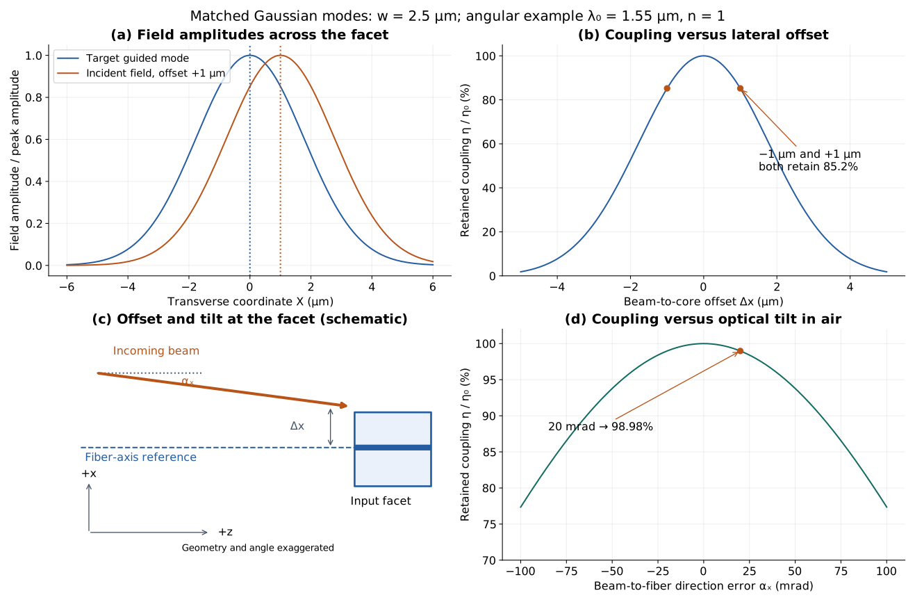
Figure 1. Field overlap and the quantities in (2). The geometry is schematic; the plots use the stated Gaussian parameters. Opposite offsets produce the same power, explaining why a single power sample cannot determine direction.

For the bench objective, use a dark-corrected, source-normalized signal:

\[F(\mathbf q)= C_{\rm det}\frac{V_{\rm out}(\mathbf q)-V_{\rm out,dark}} {V_{\rm ref}-V_{\rm ref,dark}}, \qquad \mathbf q=(x,y,z,\theta_x,\theta_y)^T.\]

The reference detector samples incident power before coupling. The constant \(C_{\rm det}\) converts detector gains and tap ratios; absolute coupling efficiency additionally requires a loss budget between the chosen input and output reference planes. Reject data when the reference signal is too small, either detector saturates, or a commanded step has not settled.

Here \(F\) is the dimensionless objective to maximize; \(V_{\rm out},V_{\rm ref}\) are output and reference detector voltages; and \(V_{\rm out,dark},V_{\rm ref,dark}\) are their voltages with the light blocked. All four voltages use the same voltage unit. \(C_{\rm det}\) is a fixed dimensionless calibration factor when both signals are voltages. The five entries of \(\mathbf q\) are the three stage translations, in length units, and the two stage rotations, in radians. Superscript \(T\) turns the written row into a column.

Example. With \(C_{\rm det}=1\), an output voltage of 1.20 V, output dark voltage of 0.02 V, reference voltage of 2.02 V, and reference dark voltage of 0.02 V give \(F=(1.20-0.02)/(2.02-0.02)=0.590\). If the source power doubles while coupling stays constant, the corresponding voltages become 2.38 V and 4.02 V, and \(F=(2.38-0.02)/(4.02-0.02)=0.590\) again. Normalization therefore keeps this source change from appearing to improve alignment.

A photodiode is authoritative only for the light delivered to it. If it collects core, cladding, and stray light, it measures their sum. Validate a measurement path that suppresses unwanted light without introducing position-dependent clipping or uncontrolled loss of the desired mode. Record polarization sensitivity and fixed downstream losses. For polarization-maintaining fiber, roll and polarization extinction may be additional alignment requirements beyond the five coordinates above.

2. What a clean SMF output can and cannot reveal

At a wavelength where only the fundamental spatial mode is guided, and after unwanted light has been removed, write

\[E_{\rm out}(X,Y)=c_{\rm g}(\mathbf q)u_{01}(X,Y), \qquad I_{\rm out}(X,Y)=|c_{\rm g}(\mathbf q)|^2|u_{01}(X,Y)|^2.\]

Here \(E_{\rm out}\) is the power-normalized output field; \(c_{\rm g}\) is its complex guided-mode amplitude; \(u_{01}\) is the fixed, unit-power output-mode profile; and \(I_{\rm out}\) is output power per unit area. With coordinates in metres, their units are \(\sqrt{\mathrm W}/\mathrm m\), \(\sqrt{\mathrm W}\), \(1/\mathrm m\), and \(\mathrm W/\mathrm m^2\), respectively. Thus \(|c_{\rm g}|^2=P_{\rm out}\), the guided output power in watts. \(c_{\rm g}\) describes optical amplitude; the mechanical dither radius introduced later is a separate quantity, \(a_{\rm d}\).

For fixed output optics and a stable fiber, the normalized image is

\[I_N(X,Y)=\frac{I_{\rm out}(X,Y)}{\iint I_{\rm out}\,dX\,dY} =\frac{|u_{01}(X,Y)|^2}{\iint |u_{01}|^2\,dX\,dY}.\]

\(I_N\) is the intensity distribution divided by its total power. It integrates to 1 and has units of inverse area; normalization does not make the local intensity density dimensionless. Its spatial shape contains no dependence on \(c_{\rm g}\). An offset launch can therefore produce the same Gaussian-looking output at lower power. Opposite offsets can produce equal power as well as equal normalized images. An intensity camera cannot identify the sign from that observation.

Example. For a Gaussian output with \(w=2.5\,\mu\mathrm m\), the normalized intensity at its center is \(I_N(0,0)=2/(\pi w^2)=0.1019\,\mu\mathrm m^{-2}\). At 1.0 mW output, the raw center intensity is \(0.1019\,\mathrm{mW}/\mu\mathrm m^2\); at 0.10 mW output, it is \(0.01019\,\mathrm{mW}/\mu\mathrm m^2\). Dividing each image by its own total power gives the same normalized center value and profile.

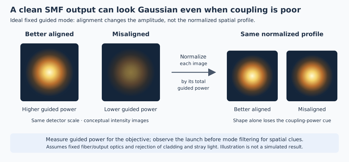
Figure 2. For an ideal clean guided output, launch alignment changes amplitude. The normalized spatial profile does not supply a correction direction.

Splitting this clean output between a near-field camera and a far-field camera does not recover the lost information: both images still scale with \(|c_{\rm g}|^2\). Their centroids may reveal motion of the output fixture or collection optics, which must not be mistaken for input-coupling error. Polarization changes, cladding modes, and parasitic interference can break this ideal picture, but are not automatically reliable alignment signals.

3. Choose an observable before choosing an algorithm

Measurement choices

Measurement	Useful information	Limitation or prerequisite
Clean output power, one sample	Value of the coupling objective	No unique correction direction from one scalar sample
Output power during known perturbations	Local slope along the perturbed coordinates	Requires signal, motion, settling or phase calibration, and averaging
Clean output intensity image	Power, output-mode quality, output-fixture diagnostics	Normalized shape usually carries no launch-error direction
Incident near- and far-field images	Beam position and angle relative to calibrated references	Reference must represent the receiving fiber, not just the camera
Residual or cladding-light image	Possible extra signatures of launch error	Experimental channel; information may vanish or change with routing
Input-facet reflection or scatter	Possible beam/facet registration or focus cues	Depends on return geometry, coating, facet angle, and ghost rejection
Pre-fiber wavefront sensor	Phase slope, curvature, and aberrations in a sampled plane	Needs amplitude/position information and a fiber-referenced target

A scalar detector does not force an optimizer to take blind random steps. Finite differences, fitted scans, and synchronous dithering all extract direction from multiple measurements under known excitation. The appropriate comparison is acquisition time and final coupling under the same starting errors and noise, rather than sensor dimensionality alone.

4. Obtain a signed gradient by mechanical dithering

Circular dither

Around a slowly varying center \((x_0,y_0)\), command a small circle:

\[x(t)=x_0+a_{\rm d}\cos\omega t,\qquad y(t)=y_0+a_{\rm d}\sin\omega t.\]

Dither motion and gradient symbols

Symbol	Definition	Units
\(t\)	Time measured from the calibrated cosine-phase reference	Seconds
\(x_0,y_0\)	Center coordinates held nearly fixed during one estimation window	Length
\(a_{\rm d}\)	Actual radius of the circular stage perturbation	Same length unit as \(x,y\)
\(f,\omega=2\pi f\)	Dither frequency and angular frequency	Hertz and radians per second
\(F_0\)	Objective evaluated at the unperturbed center	Dimensionless
\(F_x,F_y\)	Local slopes \(\partial F/\partial x,\partial F/\partial y\)	Inverse length for the dimensionless objective

Here \(a_{\rm d}\) is the actual motion amplitude in calibrated alignment coordinates, not necessarily the commanded actuator amplitude. To first order, with all other coordinates fixed,

\[F(t)\simeq F_0+a_{\rm d}F_x\cos\omega t+a_{\rm d}F_y\sin\omega t, \qquad F_x=\frac{\partial F}{\partial x},\quad F_y=\frac{\partial F}{\partial y}.\]

Both derivatives are evaluated at \((x_0,y_0)\). A positive \(F_x\) means a small positive \(x\) move increases power; a negative \(F_x\) means it decreases power. The symbol \(\simeq\) indicates that higher-order terms have been omitted. Multiplying a slope by the dither displacement gives the corresponding change in the objective.

Average over an integer number of settled cycles, denoting the average by \(\langle\cdot\rangle\):

\[\langle g\rangle= \frac{1}{T_{\rm obs}}\int_0^{T_{\rm obs}}g(t)\,dt, \qquad T_{\rm obs}=\frac{N}{f}.\]

Here \(g(t)\) is whichever measured product is being averaged; \(T_{\rm obs}\) is the observation duration in seconds; and \(N\) is a positive integer number of cycles. For sampled data, use the sample mean over complete, uniformly sampled cycles. For example, \(f=100\,\mathrm{Hz}\) and \(N=5\) give \(T_{\rm obs}=0.050\,\mathrm s\). This finite observation time is part of the measurement latency.

The gradient estimates are

(3)\[\widehat F_x=\frac{2}{a_{\rm d}}\langle F(t)\cos\omega t\rangle, \qquad \widehat F_y=\frac{2}{a_{\rm d}}\langle F(t)\sin\omega t\rangle.\]

To see why this works, multiply the first-order signal by \(\cos\omega t\). Over complete cycles the constant term averages to zero, \(\sin\omega t\cos\omega t\) averages to zero, and \(\cos^2\omega t\) averages to \(1/2\). The surviving term is \(a_{\rm d}F_x/2\); multiplication by \(2/a_{\rm d}\) returns \(F_x\). The sine channel similarly returns \(F_y\). Subtracting the mean of \(F\) before multiplication gives the same result under these complete-cycle assumptions.

The signed quadratures estimate the local gradient. Their angle, \(\operatorname{atan2}(\widehat F_y,\widehat F_x)\), gives the steepest-ascent direction in the calibrated coordinates. Their magnitude is a slope, not a distance to the optimum. A bounded update such as \(\Delta\mathbf q_{xy}=G\widehat{\nabla F}\) needs a gain matrix \(G\) with the appropriate units and stable loop dynamics. Here \(\widehat{\nabla F}=(\widehat F_x,\widehat F_y)^T\) is the estimated two-component gradient; \(\Delta\mathbf q_{xy}\) is the commanded lateral stage increment; and \(G\) is a \(2\times2\) gain matrix. If \(x,y\) are in micrometres and \(F\) is dimensionless, entries of \(G\) have units of \(\mu\mathrm m^2\). The function \(\operatorname{atan2}(v,u)\) returns the angle of a vector with horizontal component \(u\) and vertical component \(v\), including its quadrant.

Worked direction and move. For an ideal local model where the calibrated \(x,y\) coordinates equal optical offsets, let \(w=2.5\,\mu\mathrm m\), \(x_0=+1.0\,\mu\mathrm m\), and \(y_0=-0.5\,\mu\mathrm m\). Then

\[\begin{split}F_0=\exp[-(1.0^2+0.5^2)/2.5^2]=0.8187,\qquad \nabla F=-\frac{2F_0}{w^2} \begin{bmatrix}x_0\\y_0\end{bmatrix} =\begin{bmatrix}-0.262\\+0.131\end{bmatrix} \,\mu\mathrm m^{-1}.\end{split}\]

The signs call for a negative \(x\) move and a positive \(y\) move, at an angle of \(153.4^\circ\) counterclockwise from \(+x\). With \(a_{\rm d}=0.050\,\mu\mathrm m\), the cosine and sine product means are approximately \(-0.00655\) and \(+0.00328\). Applying the factors \(2/a_{\rm d}\) recovers the slopes above.

For a modest scalar gain represented by \(G=(0.50\,\mu\mathrm m^2)I_2\), where \(I_2\) is the two-dimensional identity matrix, the stage increment is \(\Delta\mathbf q_{xy}=(-0.131,+0.0655)^T\,\mu\mathrm m\). The new center is approximately \((+0.869,-0.435)\,\mu\mathrm m\), and this model predicts an objective of 0.8598. Measure the result and repeat; the gradient estimate does not itself provide a jump directly to the peak.

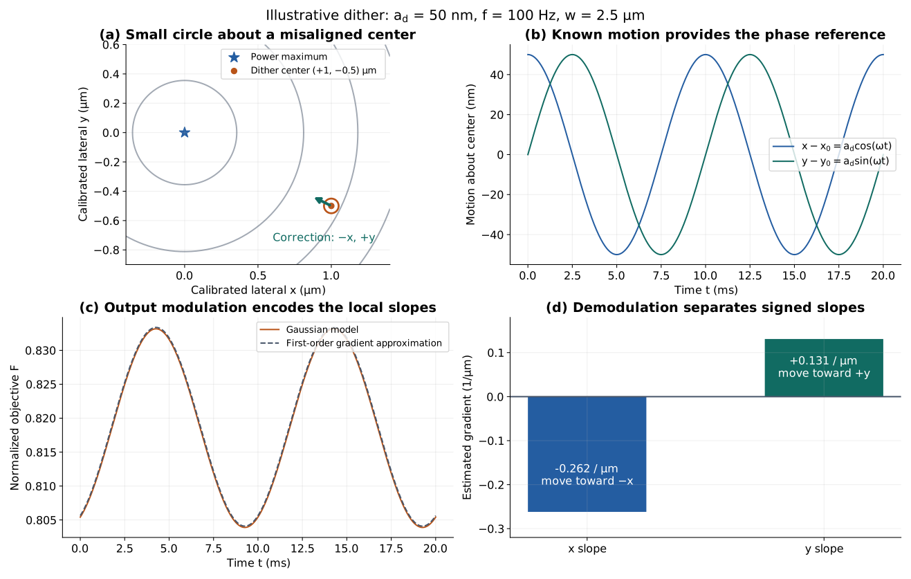
Figure 3. From known motion to a signed correction. The circle is small compared with the coupling width. The last panel separates the negative \(x\) slope from the positive \(y\) slope. The 100 Hz frequency is an illustrative choice for this model.

PI describes circular probing and gradient-search alignment in Practical Examples of Parallel Alignment Automation. The expansion here makes the small-signal assumptions explicit. It does not promise an instantaneous estimate, a global optimum, or convergence in one move.

What happens at twice the dither frequency?

Keeping the second-order terms gives

(4)\[\begin{split}\begin{aligned} F(t)\simeq{}&F_0 +a_{\rm d}(F_x\cos\omega t+F_y\sin\omega t)\\ &+\frac{a_{\rm d}^2}{4}(F_{xx}+F_{yy})\\ &+\frac{a_{\rm d}^2}{4}(F_{xx}-F_{yy})\cos 2\omega t +\frac{a_{\rm d}^2}{2}F_{xy}\sin 2\omega t. \end{aligned}\end{split}\]

The new quantities are the local curvatures: \(F_{xx}=\partial^2F/\partial x^2\), \(F_{yy}=\partial^2F/\partial y^2\), and \(F_{xy}=\partial^2F/(\partial x\partial y)\), evaluated at the dither center. They measure how a slope changes with position, with units of inverse length squared. Negative diagonal curvature describes a local peak along that coordinate; \(F_{xy}\) describes coupling between the two coordinates.

The constant term is a change in mean power. Terms multiplying \(\cos\omega t,\sin\omega t\) oscillate at \(f\) and are the fundamental. Terms multiplying \(\cos2\omega t,\sin2\omega t\) oscillate at \(2f\), the second harmonic. A detector’s mean, or DC component, is distinct from either oscillating component.

At the center of a radially symmetric peak, \(F_x=F_y=0\), \(F_{xx}=F_{yy}\), and \(F_{xy}=0\). Consequently, an ideal circular dither has no fundamental or second harmonic there. For a radial Gaussian, every point on the circle has the same power, so this statement is exact for any circle radius within that model.

In contrast, a one-axis sinusoidal dither \(x=x_0+a_{\rm d}\cos\omega t\) at a stationary point produces \(a_{\rm d}^2F_{xx}(1+\cos 2\omega t)/4\) to second order. An elliptical trajectory or unequal transverse curvatures can also produce a second harmonic. Thus, \(2f\) is not a universal signature of perfect two-axis alignment.

Example at the peak. For the normalized Gaussian with \(w=2.5\,\mu\mathrm m\), the center has \(F_0=1\), \(F_{xx}=F_{yy}=-2/w^2=-0.320\,\mu\mathrm m^{-2}\), and \(F_{xy}=0\). With \(a_{\rm d}=0.050\,\mu\mathrm m\), circular motion changes the mean to approximately 0.9996 and produces no ripple. Linear motion has a mean of approximately 0.9998 and a second-harmonic amplitude of \(-0.0002\). That is a 0.020% oscillation about the mean, with the negative sign specifying its phase relative to \(\cos2\omega t\).

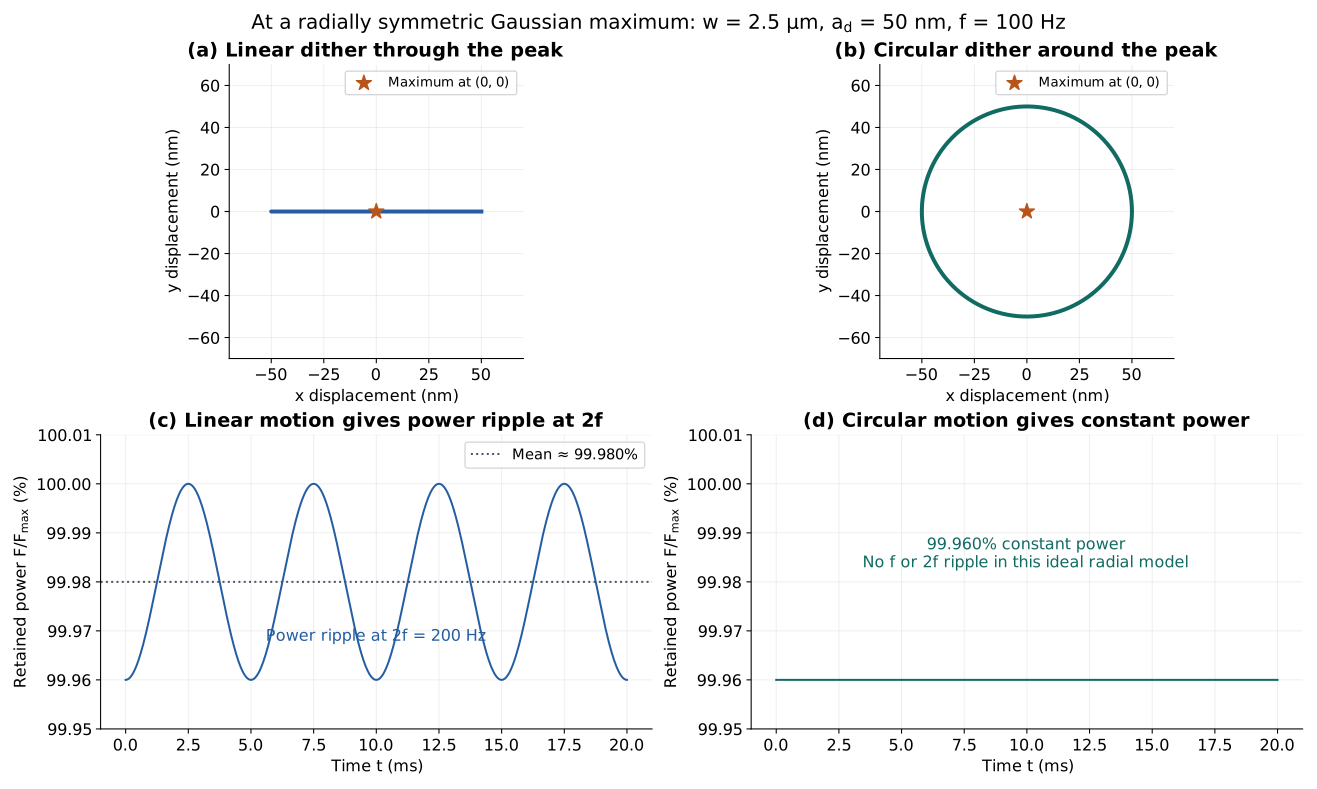
Figure 4. Why the trajectory matters. Both motions use the same 50 nm amplitude and 100 Hz frequency. Linear motion crosses the peak twice per cycle; circular motion remains at one radius. The plots are for the ideal radial model, with settled sinusoidal motion.

A vanishing fundamental alone is insufficient: there may be no light, detector saturation, a stationary minimum, or an unobserved error in another axis. Require an adequate DC signal and check that small nearby perturbations reduce the objective before declaring a maximum.

Amplitude, frequency, and practical limits

Select amplitude from the measured mode width, signal-to-noise ratio, and allowed power modulation. At the center of \(F=F_{\max}\exp[-(x^2+y^2)/w^2]\), circular dithering retains

\[\frac{F_{\rm dither}}{F_{\max}}=\exp[-a_{\rm d}^2/w^2].\]

Here \(F_{\max}\) is the stationary value at the peak, and \(F_{\rm dither}\) is the value measured while traversing the centered circle. For this radial model it is constant along the circle, so its instantaneous value and mean are identical. For \(w=2.5\,\mu\mathrm{m}\) and \(a_{\rm d}=50\,\mathrm{nm}=0.050\,\mu\mathrm m\), substitution gives \(\exp[-(0.050/2.5)^2]=0.999600\), or 99.960%, a 0.040% penalty. A small penalty does not establish that the modulation is measurable on a particular instrument.

Choose frequency from the loaded stage transfer function, detector bandwidth, sampling rate, and total latency. Measure the actual amplitude and phase of both axes; compensate phase lag and cross-axis motion before interpreting the quadratures. Sample well above the frequencies being demodulated and filter against aliasing. Average long enough to resolve the signal while keeping the center nearly stationary during estimation. There is no universal nanometer amplitude or frequency range that fits all piezo stages, stepper stages, payloads, and detector gains.

When smooth periodic motion is unavailable, use settled central differences instead:

\[\widehat F_j = \frac{F(\mathbf q+h_j\mathbf b_j)-F(\mathbf q-h_j\mathbf b_j)}{2h_j}.\]

Here \(j\) selects one stage coordinate; \(\mathbf b_j\) is a column vector with 1 in that coordinate and 0 elsewhere; and \(h_j>0\) is a chosen perturbation in that coordinate’s units. \(\widehat F_j\) estimates its slope, in inverse length for a translation or inverse radians for a rotation. The two measurements are taken at settled positions equally spaced about \(\mathbf q\).

Example. A step \(h_x=0.10\,\mu\mathrm m\) giving \(F(x+h_x)=0.79\) and \(F(x-h_x)=0.84\) yields \(\widehat F_x=(0.79-0.84)/(2\times0.10) =-0.25\,\mu\mathrm m^{-1}\). Power rises toward negative \(x\). The two samples bracket the current point, so source drift and backlash between them can bias the estimate.

Pair measurements closely in time, normalize source power, and account for backlash. Extend to focus and angular coordinates sequentially, or use separable dither frequencies only after checking harmonic overlap and mechanical coupling. Dither is a local tracking method: a bounded coarse scan is still needed when there is no measurable first light.

5. Place spatial sensors where information survives

Incident near field and far field

Tap the incident beam before the fiber. Relay a plane conjugate to the input facet onto one camera and a calibrated Fourier plane onto another. In an ideal uncoupled paraxial arrangement,

\[\Delta x_{\rm image}=M\Delta x_{\rm facet},\qquad \Delta x_{\rm Fourier}\simeq f_{\rm F}\Delta\alpha_x,\]

with analogous equations for \(y\). Here \(M\) is signed magnification and \(f_{\rm F}\) is the effective Fourier-plane focal length. General relays mix position and angle, so calibrate their full response rather than assuming these two ideal equations.

Position and angle measurements

Symbol	Definition	Units
\(\Delta x_{\rm image}\)	Near-field camera centroid displacement from the registered fiber reference	Physical length on the sensor
\(\Delta x_{\rm facet}\)	Incident-beam displacement from the fiber reference at the facet	Physical length at the facet
\(M\)	Sensor displacement divided by corresponding facet displacement	Dimensionless; its sign includes image inversion
\(\Delta x_{\rm Fourier}\)	Fourier-plane centroid displacement from the aligned direction reference	Physical length on the sensor
\(f_{\rm F}\)	Calibrated focal length converting angular change into sensor displacement	Length
\(\Delta\alpha_x\)	Optical beam-direction change toward \(+x\) from the calibrated reference	Radians; this is an optical change, not a stage rotation command

The near-field camera answers where the beam is; the Fourier-plane camera answers which way it points. These measurements use distinct reference planes, even when the cameras have identical sensors.

Example. Let both cameras have pixel pitch \(p=5\,\mu\mathrm m/\mathrm{pixel}\), where \(p\) converts a centroid displacement in pixels to physical sensor length. In the near-field branch, \(M=+40\) and a displacement of +8 pixels give \(\Delta x_{\rm image}=8\times5=40\,\mu\mathrm m\), hence \(\Delta x_{\rm facet}=40/40=+1.0\,\mu\mathrm m\). In the Fourier branch, a +10 pixel displacement with \(f_{\rm F}=50\,\mathrm{mm}=50{,}000\,\mu\mathrm m\) gives \(\Delta\alpha_x=(10\times5)/50{,}000=0.001\,\mathrm{rad} =+1.0\,\mathrm{mrad}\). Figure 5 illustrates these conversions.

The reference must be tied to the receiving fiber. Options include an illuminated facet image, a removable reference target, or a suitable back-launched guided mode. If the fiber moves while a pre-fiber camera sees only the stationary incident beam, that camera alone cannot detect the resulting relative error. Two centroid measurements can constrain four transverse coordinates; focus generally needs extra information, such as curvature or a scan. A single waist-size image does not usually distinguish positive from negative defocus.

Residual and cladding-light imaging

Imaging a wider region of the output facet may reveal light outside the desired guided mode. For a dark-corrected residual region, possible features are

\[S_x=\frac{P_R-P_L}{P_R+P_L},\qquad S_y=\frac{P_T-P_B}{P_T+P_B}.\]

\(P_R,P_L\) are the integrated powers in the right and left halves of a selected residual-light region, and \(P_T,P_B\) are the powers in its top and bottom halves. Use the same background subtraction, gain, and spatial mask for each partition. The central region selected for exclusion contributes to none of these sums. Power units can be watts or milliwatts, provided numerator and denominator use the same unit. Calibrated proportional camera counts also give the same ratios.

\(S_x,S_y\) are dimensionless asymmetries between -1 and +1 for nonnegative powers. Positive \(S_x\) means more residual light on the right; positive \(S_y\) means more on the top. Those signs describe the image, and a measured calibration must determine the corresponding mechanical correction.

Example. With \(P_R=0.60\,\mathrm{mW}\) and \(P_L=0.40\,\mathrm{mW}\), \(S_x=(0.60-0.40)/(0.60+0.40)=+0.20\). With \(P_T=0.55\,\mathrm{mW}\) and \(P_B=0.45\,\mathrm{mW}\), \(S_y=+0.10\). If independent calibration established \(S_x-S_{x,*}\simeq K_x\Delta x\), with a target asymmetry \(S_{x,*}=0\) and slope \(K_x=+0.20\,\mu\mathrm m^{-1}\), the observed \(S_x\) estimates \(\Delta x=+1.0\,\mu\mathrm m\) within that calibration region. A measured negative \(K_x\) would reverse the interpretation. This example assumes such a calibration; it does not establish that a particular fiber produces that response.

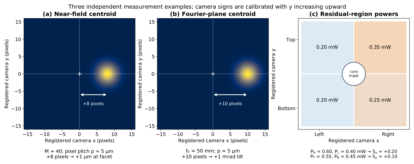
Figure 5. Three independent illustrative measurements. The camera panels mark the registered zero and measured displacement. The residual panel defines the regions whose integrated powers enter \(S_x,S_y\); it represents region totals, not a simulated cladding-light distribution.

Only use them above a defined denominator/noise threshold. The relations \(S_x\propto\Delta x\) and \(S_y\propto\Delta y\) are hypotheses to test, not general fiber laws. Radiation can leave near the launch end; cladding light can be attenuated by coating, bends, length, and stripping. Interference may scramble an apparent sign when the fiber is rerouted. The guided fundamental mode itself extends into the cladding; that ordinary mode tail is not a separate cladding-mode error channel. Even a camera region centered on the core does not guarantee that only the guided core mode contributes to its pixels.

Keep this exploratory channel separate from the validated guided-power objective. Clamp the output fixture and collection optics during input scans so that image motion does not simply report mechanical motion at the far end. Repeat calibration after realistic routing and temperature changes before considering production feedback.

Facet reflection and wavefront sensing

An input-side return path can image the facet, reflected spot, or scatter when the far end is inaccessible. Its usefulness depends on facet angle, anti-reflection coating, core visibility, and separation of unwanted reflections. Specular reflection from a uniform flat facet alone does not identify the core center. Treat any inferred coupling metric as a proxy until checked against actual guided transmission on a representative setup.

A Shack–Hartmann sensor measures local wavefront slopes from lenslet-spot displacements; see Thorlabs’ Adaptive Optics technical whitepaper. It can help measure tilt, curvature, and aberration of the incident beam. However, translating a collimated flat-wavefront beam need not tilt its wavefront. Lateral registration requires an intensity centroid or another position reference. The target is the field matched to the fiber after propagation through the coupling optics; making an arbitrary sampled wavefront flat is not by itself a coupling optimum.

6. Calibrate a multi-axis spatial controller

What the response matrix measures

Let \(\mathbf s\) contain image features such as registered centroids, wavefront curvature, or validated residual asymmetries. Record the target \(\mathbf s_*\) at an independently verified coupling maximum and define \(\mathbf e=\mathbf s-\mathbf s_*\). Near that point,

\[\Delta\mathbf s\simeq J\Delta\mathbf q, \qquad J_{ij}\simeq \frac{s_i(\mathbf q_*+h_j\mathbf b_j) -s_i(\mathbf q_*-h_j\mathbf b_j)}{2h_j}.\]

The first relation says that a small stage move produces a predictable change in the measured features. The second estimates one response coefficient by deliberately moving an axis in each direction, just as the power-gradient central difference did earlier.

Response and correction symbols

Symbol	Definition	Size or units
\(\mathbf q,\mathbf q_*\)	Current stage coordinates and target coordinates at verified optimum	Five entries: three lengths and two angles
\(\mathbf s,\mathbf s_*\)	Current measured features and features recorded at that target	\(m\) entries; \(m\) is the number of selected features
\(\mathbf e=\mathbf s-\mathbf s_*\)	Current feature error relative to the target	Same units as the corresponding features
\(\Delta\mathbf q,\Delta\mathbf s\)	Small changes of the stage vector and feature vector	Same units as their corresponding entries
\(J\)	Local response matrix, often called the Jacobian	\(m\times5\); each entry is feature units per coordinate unit
\(J_{ij},s_i\)	Response of feature \(i\) to coordinate \(j\), and feature \(i\)	For example, pixels per micrometre for a centroid/translation pair
\(h_j,\mathbf b_j\)	Calibration step and coordinate-selection vector defined in Section 4	Length or angle, and a dimensionless five-entry vector

The ideal local correction is \(\Delta\mathbf q=-\gamma J^+\mathbf e\), where \(0<\gamma\leq1\) damps the step. The minus sign follows from the stated error convention. Here \(J^+\) is the pseudoinverse: the matrix that converts measured feature error into a least-squares stage-error estimate. It is an ordinary inverse when the response is square and nonsingular. It has size \(5\times m\), with coordinate units per feature unit. The dimensionless factor \(\gamma\) chooses how much of the estimated correction to apply. More features do not guarantee independent information: two physically different errors can produce the same image.

Worked two-axis calibration and correction

For a small example, hold the other three axes fixed and use two camera centroid features. Set \(\mathbf q_*=(0,0)^T\,\mu\mathrm m\) and \(\mathbf s_*=(0,0)^T\) pixels by choosing their aligned reference positions as zero. Move each stage axis by \(h_x=h_y=0.25\,\mu\mathrm m\):

Hypothetical measured calibration data

Stage perturbation about target	Feature 1 displacement (pixels)	Feature 2 displacement (pixels)
\(x=+0.25\,\mu\mathrm m\)	+1.00	+0.25
\(x=-0.25\,\mu\mathrm m\)	-1.00	-0.25
\(y=+0.25\,\mu\mathrm m\)	+0.25	+0.75
\(y=-0.25\,\mu\mathrm m\)	-0.25	-0.75

For example, \(J_{11}=[1.00-(-1.00)]/(2\times0.25) =4.00\,\mathrm{pixels}/\mu\mathrm m\). Computing all four entries gives

\[\begin{split}J=\begin{bmatrix}4&1\\1&3\end{bmatrix} \frac{\mathrm{pixels}}{\mu\mathrm m}.\end{split}\]

Its first column means a +1 micrometre \(x\) move changes the two features by \((+4,+1)\) pixels. Its second column means a +1 micrometre \(y\) move changes them by \((+1,+3)\) pixels. The off-diagonal entries express cross-axis coupling: neither feature depends on just one stage coordinate.

Now measure \(\mathbf e=(7,-1)^T\) pixels and choose \(\gamma=0.5\). Solving for the estimated stage error and applying the correction gives

\[\begin{split}J^{-1}\mathbf e= \frac{1}{11}\begin{bmatrix}3&-1\\-1&4\end{bmatrix} \begin{bmatrix}7\\-1\end{bmatrix} =\begin{bmatrix}2\\-1\end{bmatrix}\,\mu\mathrm m, \qquad \Delta\mathbf q= \begin{bmatrix}-1\\+0.5\end{bmatrix}\,\mu\mathrm m.\end{split}\]

Thus the command is negative \(x\), positive \(y\). The predicted new feature error is \(\mathbf e+J\Delta\mathbf q=(3.5,-0.5)^T\) pixels, half its initial value. Figure 6 shows the move in both coordinate systems. The values illustrate the calculation; a real machine must measure its own response matrix and verify the actual post-move power.

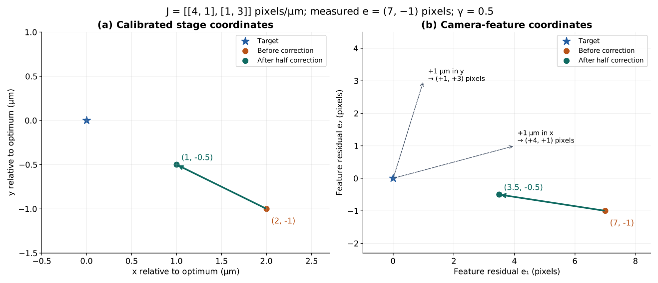
Figure 6. The same correction expressed as stage motion and camera feature change. Dashed arrows on the right show the two measured response columns. The green move applies half the inferred correction.

Optional: scale coordinates and account for noise

Before inverting, scale coordinates and account for feature noise. With diagonal coordinate scales \(Q\), measured feature covariance \(C_s\), and a regularized inverse square root of that covariance, define

\[ \begin{align}\begin{aligned}A=C_s^{-1/2}JQ,\qquad \mathbf r=C_s^{-1/2}\mathbf e,\\\Delta\mathbf q= -\gamma Q(A^TA+\rho^2 I)^{-1}A^T\mathbf r.\end{aligned}\end{align} \]

Symbols in the noise-scaled correction

Symbol	Definition and purpose	Size or units
\(Q\)	Diagonal matrix of positive reference step sizes; makes stage changes comparable	\(5\times5\); diagonal entries have the corresponding coordinate units
\(C_s\)	Covariance of repeated stationary feature measurements; characterizes measurement noise	\(m\times m\); entry \(i,j\) has feature \(i\) units times feature \(j\) units
\(C_s^{-1/2}\)	Inverse square root of covariance; divides independent features by their noise and accounts for correlation	Maps feature quantities into dimensionless noise-scaled quantities
\(A=C_s^{-1/2}JQ\)	Response to normalized stage steps, expressed relative to feature noise	\(m\times5\), dimensionless
\(\mathbf r=C_s^{-1/2}\mathbf e\)	Feature error expressed relative to measurement noise	\(m\) entries, dimensionless
\(\rho\)	Regularization strength; reduces sensitivity to weakly measured directions	Nonnegative and dimensionless; distinct from optical wavelength \(\lambda_0\)
\(I\)	Identity matrix matching the number of active coordinates	\(5\times5\) for all five axes
Superscripts \(T\) and \(-1\)	Matrix transpose and matrix inverse, respectively	Operations, not measured quantities

The formula finds a stage correction that reduces noise-scaled feature error while penalizing large normalized moves. Increase \(\rho\) to suppress corrections along weak response directions; this usually leaves more residual error. Choose it from calibration noise and validation, rather than treating regularization as extra sensor information.

For the two-axis example, suppose the two features have independent noise with standard deviation 0.5 pixels, and use reference steps of 1 micrometre. Then \(C_s=(0.5\,\mathrm{pixels})^2 I_2\), \(Q=(1\,\mu\mathrm m)I_2\), \(A=\left[\begin{smallmatrix}8&2\\2&6\end{smallmatrix}\right]\), and \(\mathbf r=(14,-2)^T\). The standard deviation is the typical noise spread of a feature; its square is the corresponding diagonal covariance entry. With \(\gamma=0.5\), substitution gives:

Effect of regularization on the same measured error

\(\rho\)	Stage correction \(\Delta\mathbf q\) (micrometres)	Predicted feature error after move (pixels)
0	\((-1.000,+0.500)^T\)	\((+3.500,-0.500)^T\)
2	\((-0.903,+0.393)^T\)	\((+3.782,-0.725)^T\)

Inspect the singular values of \(A\): these are the response strengths for independent combinations of normalized stage coordinates, measured in units of feature noise. In the two-axis example they are 9.24 and 4.76, so both directions have a measurable response in this hypothetical noise model. A singular value near zero indicates a stage-error combination that the selected features scarcely distinguish from noise. Recovering all five coordinates requires five sufficiently strong independent responses; regularization cannot create a missing measurement. Retain only supported directions, bound each move to the validated calibration region, remeasure, and accept a step only when the guided-power check supports it. A calibrated camera loop can then hand over to fine power optimization.

Image regression or machine learning should face the same observability test. Split validation by fiber/assembly and session, not just adjacent frames from one scan. Include unseen combined-axis offsets and routing conditions, compare against the local Jacobian baseline, and fall back to power search outside the validated range. A model cannot recover a sign that ideal single-mode propagation has physically removed.

7. A practical architecture and operating sequence

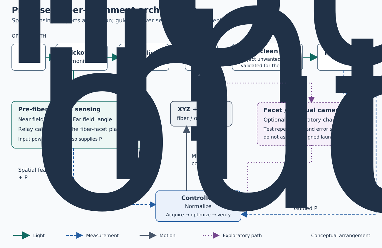
Figure 7. Proposed measurement architecture. Spatial references must be registered to the fiber, and the main power channel must reject unwanted light.

In this diagram, \(P_{\rm in}\) is incident optical power sampled before the coupling optics, and \(P_{\rm out}\) is the desired guided power measured after the validated output path. Both are powers in watts or milliwatts; their ratio is dimensionless. The detector voltages in Section 1 are calibrated proxies for these powers. Thus \(P_{\rm out}/P_{\rm in}=0.60\) for 3.0 mW output and 5.0 mW input, before any separately accounted losses between reference planes.

Start with the guided-power channel and add spatial sensing when its measured acquisition benefit justifies the extra calibration.

1. Establish references. Set wavelength, polarization, mode-field size, facet plane, detector gains, input-power reference, and stage limits. Establish approximate mode matching before a fine position search.

2. Find first light. Use facet/beam registration or a bounded raster or spiral scan. Set a detection threshold above measured dark/background fluctuations. A flat noise floor is not an alignment maximum.

3. Optimize locally. Use fitted scans, central differences, or dither on the available axes. Revisit lateral alignment after focus or angle moves because real mechanisms couple these motions.

4. Validate the peak. Check neighboring points, adequate guided power, detector linearity, and repeatability. Reduce or stop dither and measure the stationary result separately from the modulated average.

5. Verify the finished assembly. Recheck after locking, adhesive cure, fixture release, and a specified settling interval. Log retained coupling and polarization performance where applicable.

6. Track or reacquire. For continuous operation, limit tracking motion and trigger reacquisition when signal or confidence is lost. Avoid integrating noise into unlimited stage travel.

8. Feasibility experiment and acceptance criteria

Test the sensor before developing a complex controller. Record the fiber type, wavelength, length, routing, stripping arrangement, optics, stage pivot, detector bandwidths, camera exposure, and coordinate signs.

1. Find a reproducible power maximum and estimate the coupling width of each movable axis. Select perturbations from those widths and the actual stage resolution; label all scan ranges and units.

2. Record repeated stationary samples to estimate feature covariance, power noise, and drift. Fix exposure and gain, subtract background, avoid saturation, and keep raw images as well as normalized images.

3. Scan positive and negative offsets about the optimum. Randomize scan order, revisit the center, and repeat in both motion directions to expose drift and backlash. Collect settled timestamps, actual stage positions, reference power, and validated guided power together.

4. Test combinations of lateral, focus, and angular errors. Estimate the scaled response matrix and compare feature changes with their noise. Identical images at opposite offsets are an ambiguity, not a training problem solved by collecting more copies of the same data.

5. Repeat after remounting or rerouting and across the expected operating conditions. Check that a model trained in one session retains its direction and scale in another.

6. Compare complete closed-loop runs from held-out starting positions against a power-only baseline. Include acquisition, averaging, settling, and failed retries in the timing.

Define pass/fail limits before the comparison

Quantity	What to measure	Decision it supports
Capture range and success rate	Convergence fraction over a declared starting-position region	Whether coarse acquisition is adequate
Final coupling	Stationary guided power relative to a verified reference maximum	Whether speed sacrifices optical performance
Acquisition time	Median and upper-percentile time, including retries	Whether the added sensor improves throughput
Observability and direction	Scaled singular values and held-out correction-direction errors	Which axes may safely use spatial feedback
Dither penalty	Mean power reduction and modulation during tracking	Whether the tracking signal meets the optical budget
Robustness after assembly	Coupling after locking, cure, routing, and thermal settling	Whether the alignment survives the real process

If normalized clean-output images remain identical while power changes, use power-based optimization and reserve the profiler for output-quality diagnostics. If extra spatial channels reliably predict corrections, use them within their demonstrated capture region and retain guided power as the final acceptance measurement.

9. Using KrakenOS and reading further

Use KrakenOS to study coupling-optic geometry, stage perturbations, clearance, and Gaussian-beam propagation. A geometrically small ray spot or rays landing inside the core does not establish SMF efficiency; a field-overlap calculation is required. The scalar Gaussian overlap tools described in Gaussian Beam Propagation provide a starting point for idealized studies. They do not by themselves model cladding-mode transport, motion dynamics, or a production alignment controller.

• Fiber Coupling and Interferometer Alignment gives related bench procedures for fiber injection and interferometers.

• Reference Axis and Mirror Steering develops the distinction between position and angle alignment.

• Newport: Fiber Optic Coupling provides the mode-matching basis for the coupling objective.

• PI: Practical Examples of Parallel Alignment Automation describes practical gradient-search alignment.

• Thorlabs / Boston Micromachines: Adaptive Optics technical whitepaper explains wavefront-sensor measurements and correction.

The Gaussian overlap example, harmonic expansion, and calibration equations on this page are worked analytical models with their assumptions stated alongside them. Residual-light sensing and image regression remain experimental options to be evaluated with the procedure above.

The analytical plots and measurement diagrams are reproducible with docs/generate_active_alignment_figures.py. For example, from the repository root run python docs/generate_active_alignment_figures.py --preview-dir /tmp/alignment-previews. The generator uses NumPy and Matplotlib and checks the displayed coupling and correction examples before writing the SVG assets.