7.10 Example — Doublet Lens Pupil
PDF section 7.10. Source script: KrakenOS/Examples/Examp_Doublet_Lens_Pupil.py.
Uses PupilCalc Tool to read the entrance- and exit-pupil parameters of the doublet with an inserted aperture stop, then samples a fan pattern at field ±2° and traces it through the system.
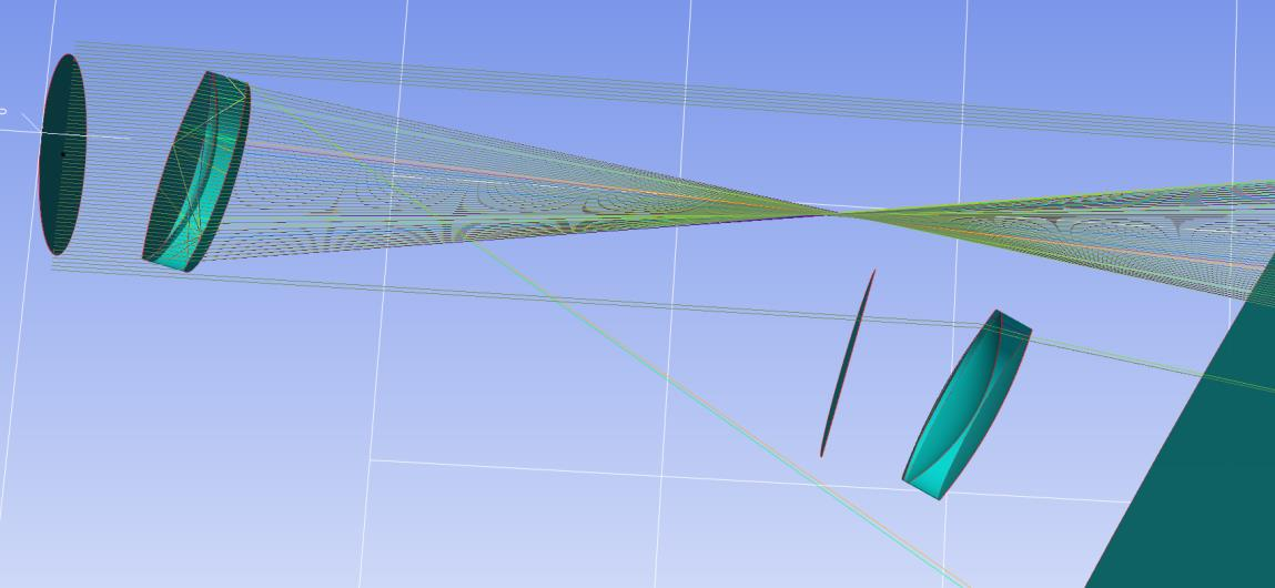
Figure 17. Beams generated by PupilCalc — the position of the
aperture-stop surface determines the pupil layout.
#!/usr/bin/env python3
# -*- coding: utf-8 -*-
"""
Example: Doublet Lens with Pupil Calculation

This script demonstrates how to simulate a doublet lens system with pupil calculation using KrakenOS.
The system includes:
  - Object Plane (source)
  - First lens surface (convex, BK7)
  - Second lens surface (concave, F2)
  - Air gap (with modified thickness)
  - Pupil surface (defining the pupil of the system)
  - Image Plane (detector)

The script performs a pupil calculation using the PupilCalc tool and then generates a ray pattern based on the pupil.
It traces the rays for two field orientations (FieldY = 2.0 and FieldY = -2.0) and finally displays a 2D visualization.

Author: Joel Herrera V.
Date: 10/03/2025
"""

from importlib import metadata

# =============================================================================
# Check if KrakenOS is installed.
# If not, assume that the code is run from a downloaded GitHub folder and add the relative path.
# =============================================================================
required = {'KrakenOS'}
installed = {dist.metadata["Name"] for dist in metadata.distributions() if dist.metadata.get("Name")}
missing = {pkg for pkg in required if pkg not in installed}

if missing:
    print("KrakenOS is not installed. Using local GitHub folder.")
    import sys
    sys.path.append("../..")  # Adjust this path if necessary

import KrakenOS as Kos  # Import KrakenOS for optical simulation

# =============================================================================
# Define the optical surfaces for the doublet lens system with pupil.
#
# The system is composed of:
#   - Object Plane: Source plane (flat, air)
#   - First Lens Surface: Convex surface made of BK7
#   - Second Lens Surface: Concave surface made of F2
#   - Air Gap: Modified air gap between lens and pupil/image plane
#   - Pupil: Pupil surface with specific displacement and nominal positions
#   - Image Plane: Detector where the final image is formed
# =============================================================================

# Object Plane (Source)
P_Obj = Kos.surf()
P_Obj.Rc = 0.0
P_Obj.Thickness = 100          # Distance to the next surface (mm)
P_Obj.Glass = "AIR"
P_Obj.Diameter = 30.0
P_Obj.Name = "P_Obj"

# First Lens Surface (convex, BK7)
L1a = Kos.surf()
L1a.Rc = 9.284706570002484E+001  # Convex curvature
L1a.Thickness = 6.0              # Lens thickness (mm)
L1a.Glass = "BK7"
L1a.Diameter = 30.0
L1a.Axicon = 0                  # No axicon effect

# Second Lens Surface (concave, F2)
L1b = Kos.surf()
L1b.Rc = -3.071608670000159E+001  # Concave curvature
L1b.Thickness = 3.0              # Separation between surfaces (mm)
L1b.Glass = "F2"
L1b.Diameter = 30

# Air Gap before pupil and image plane
L1c = Kos.surf()
# The thickness is set to (9.737604742910693E+001 - 40) mm to account for design constraints.
L1c.Rc = -7.819730726078505E+001
L1c.Thickness = 9.737604742910693E+001 - 40
L1c.Glass = "AIR"
L1c.Diameter = 30

# Pupil Surface
pupil = Kos.surf()
pupil.Rc = 0
pupil.Thickness = 40.0         # Thickness of the pupil element (mm)
pupil.Glass = "AIR"
pupil.Diameter = 3
pupil.Name = "Pupil"
pupil.DespY = 0.0              # Y displacement (if any)
pupil.Nm_Pos = [-10, 10]       # Name label position

# Image Plane (Detector)
P_Ima = Kos.surf()
P_Ima.Rc = 0.0
P_Ima.Thickness = 0.0
P_Ima.Glass = "AIR"
P_Ima.Diameter = 20.0
P_Ima.Name = "P_Ima"
P_Ima.Nm_Pos = [-10, 10]       # Name label position

# =============================================================================
# Assemble the optical surfaces into a system.
#
# The order of surfaces in list A defines the optical sequence.
# =============================================================================
A = [P_Obj, L1a, L1b, L1c, pupil, P_Ima]
config_1 = Kos.Setup()
Doublet = Kos.system(A, config_1)
RayKeeper = Kos.raykeeper(Doublet)  # Container to store traced rays

# =============================================================================
# Pupil Calculation
#
# Use the PupilCalc tool to compute pupil parameters.
#
# Parameters:
#  - sup: Index of the surface where the pupil is defined (here, 4, as pupil is the 5th surface)
#  - W: Wavelength (0.4)
#  - AperType: Type of aperture ("STOP")
#  - AperVal: Aperture value (3)
# =============================================================================
W = 0.4        # Wavelength
sup = 4        # Surface index for pupil (0-based indexing: pupil is the 5th surface)
AperVal = 3    # Aperture value
AperType = "STOP"  # Aperture type

Pup = Kos.PupilCalc(Doublet, sup, W, AperType, AperVal)

# Print pupil parameters for analysis
print("Input pupil radius:")
print(Pup.RadPupInp)
print("Input pupil position:")
print(Pup.PosPupInp)
print("Output pupil radius:")
print(Pup.RadPupOut)
print("Output pupil position:")
print(Pup.PosPupOut)
print("Output pupil position relative to the focal plane:")
print(Pup.PosPupOutFoc)
print("Output pupil orientation:")
print(Pup.DirPupSal)
print("Airy disk diameter at focal distance (micrometers):")
print(Pup.FocusAiryRadius)

# Extract the output pupil orientation (direction cosines)
[L, M, N] = Pup.DirPupSal
print("Pupil output direction cosines:", L, M, N)

# =============================================================================
# Generate the ray pattern based on the pupil calculation.
#
# The pupil configuration is used to generate a set of rays on the image plane.
# Two field patterns are generated: one for FieldY = 2.0 and one for FieldY = -2.0.
# =============================================================================

# First field pattern: FieldY = 2.0
Pup.Samp = 7           # Number of samples
Pup.Ptype = "fany"      # Pattern type (e.g., fan-like distribution)
Pup.FieldType = "angle" # Field defined in terms of angle
Pup.FieldY = 2.0       # Field parameter (positive Y direction)
x, y, z, L, M, N = Pup.Pattern2Field()  # Generate field pattern

# Trace rays for the first pattern
for i in range(len(x)):
    pSource_0 = [x[i], y[i], z[i]]   # Ray origin
    dCos = [L[i], M[i], N[i]]         # Ray direction cosines
    Doublet.Trace(pSource_0, dCos, W)
    RayKeeper.push()

# Second field pattern: FieldY = -2.0
Pup.FieldY = -2.0
x, y, z, L, M, N = Pup.Pattern2Field()  # Generate field pattern for negative FieldY
for i in range(len(x)):
    pSource_0 = [x[i], y[i], z[i]]
    dCos = [L[i], M[i], N[i]]
    Doublet.Trace(pSource_0, dCos, W)
    RayKeeper.push()

# =============================================================================
# Display the final ray tracing result.
#
# You can choose between 3D and 2D visualization. Here, a 2D plot is generated.
# =============================================================================
# Uncomment the following line for 3D visualization:
# Kos.display3d(Doublet, RayKeeper, 2)
Kos.display2d(Doublet, RayKeeper, 0, 1)