Case Study 2: Focus A Finite Machine-Vision Lens

Goal

This case study starts from the measured 150 mm machine-vision lens preset and uses a deliberately wrong sensor position to show a complete sequential design loop:

• load a finite-conjugate lens;

• make a poor first Spot and MTF analysis;

• choose the correct optimization variable;

• run a best-focus solve;

• verify that Spot and MTF improve.

The point is not to redesign the lens prescription. The lens is treated as a measured black-box machine-vision lens. The user is only recovering the correct sensor/image distance for a finite object.

The screenshots in this tutorial are generated from the live Tk UI with:

python -m KrakenOS.UI.capture_machine_vision_case_study_screenshots

The analysis screenshots are area-of-interest crops from the Matplotlib plot canvas so the result is readable during a presentation.

Load The Finite Lens

1. Start the UI with python -m KrakenOS.UI.layout_editor.

2. In the top menu, choose the machine-vision preset Machine Vision 150Mm Measured.

3. Confirm the left/source panel is in finite-object mode:

   • Object Mode = Finite;

   • Aperture = FNO;

   • FNO = 5.6;

   • Field Type = Object Height;

   • Field Value = 0;

   • Field Count = 1.

This is the on-axis setup. Use it first because focus must be correct before a wide-field comparison is meaningful.

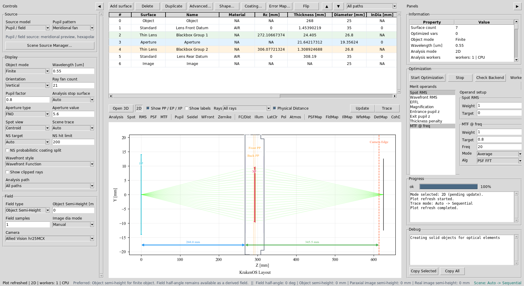
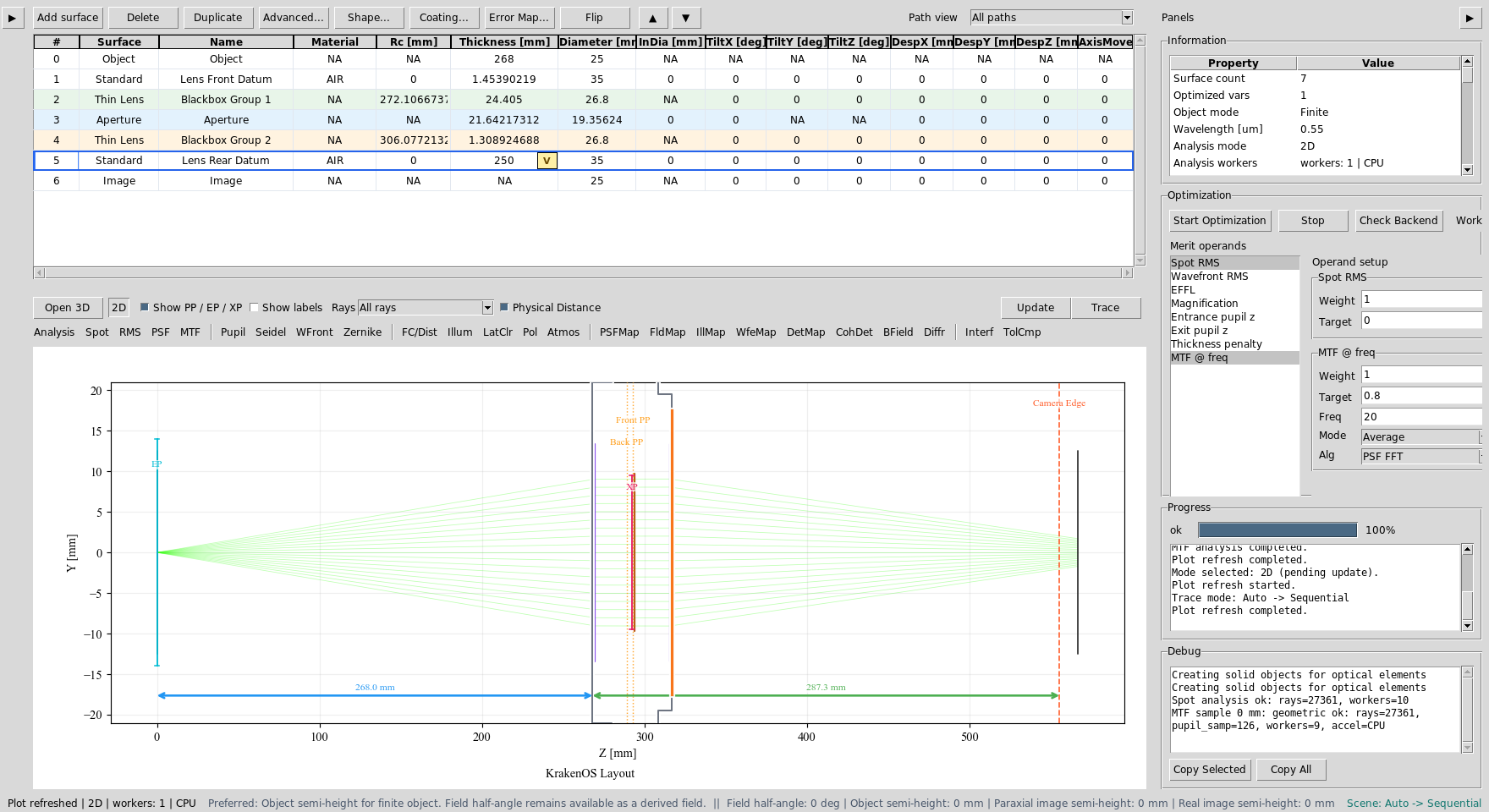
The measured finite-conjugate machine-vision lens is loaded. The table uses object distance, lens front/rear datums, black-box lens groups, aperture, and Image rows.

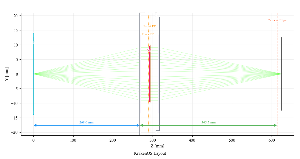
Initial 2D layout: the finite object launches into the measured lens group and ends at the Image plane / sensor position.

Make A Bad First Analysis

In the table, find row S5 Lens Rear Datum. This row thickness is the air gap from the rear lens datum to the Image row, so it behaves like the sensor position.

For the bad starting point, type:

S5 Thickness = 250

Then click Spot and Update.

The on-axis spot is intentionally bad. In the generated screenshot, the spot RMS is about 1.21 mm because the sensor is much too close to the lens. Spot diagrams use equal X/Y physical scale, so circular blur stays circular instead of being stretched by the plot panel.

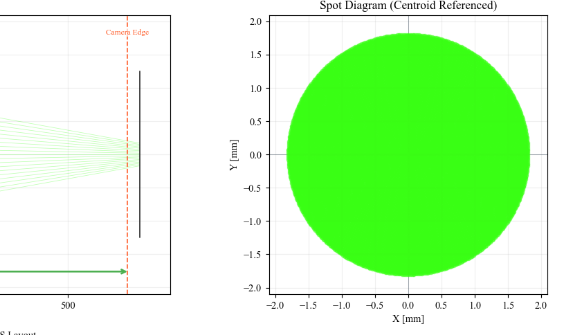
Defocused Spot AOI: the sensor is at 250 mm instead of near focus.

Click MTF and Update. Use MTF @ freq = 20 cycles/mm and Alg = PSF FFT in the Optimization panel. The defocused geometric MTF is nearly gone at this frequency.

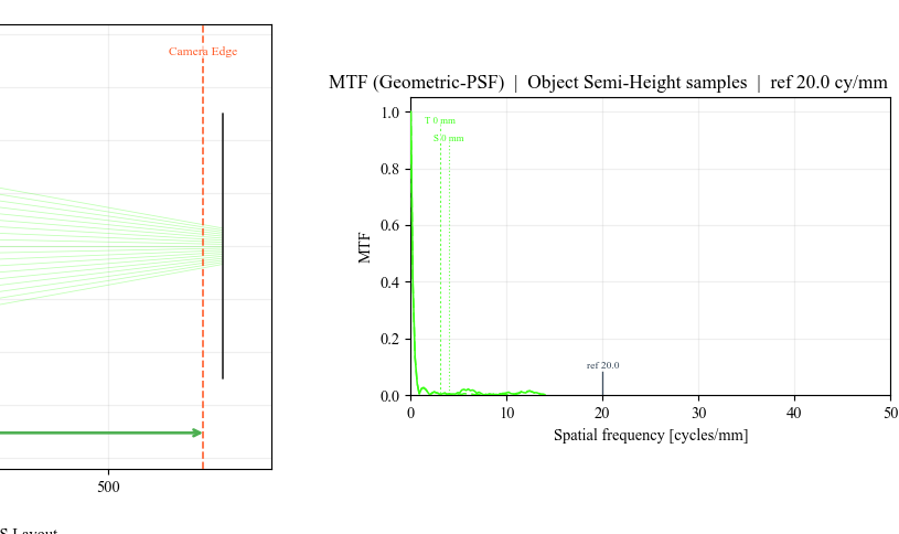
Defocused MTF AOI: at 20 cycles/mm the average geometric MTF is only around 0.008 for this deliberate sensor error.

Choose The Right Variable

The optimizer needs a variable. For this workflow the variable is not a lens radius or glass. It is the sensor distance:

1. Right-click the S5 Lens Rear Datum Thickness cell.

2. Choose Optimization / Solves -> Select Thickness for optimization.

3. Right-click the same cell again and choose Set bounds....

4. Use a practical focus-search range, for example:

240, 330

Keep the Spot RMS merit operand selected with target 0. This tells the UI: move only the image distance until the on-axis spot is minimized.

S5 Thickness is the focus variable. Spot RMS is the target metric.

Run The Focus Solve

Use either workflow below.

Workflow A: best-focus solve

This is the most direct click-through path:

1. Right-click S5 Lens Rear Datum Thickness.

2. Choose Optimization / Solves -> Best Focus Solve.

3. Accept the result and click Update.

For this case study the solve moves the sensor to about:

S5 Thickness ~= 308.3 mm

The on-axis spot RMS improves from about 1.21 mm to about 0.0022 mm.

Workflow B: general optimizer

This demonstrates the same idea through the Optimization panel:

1. Keep only S5 Thickness marked as a variable.

2. Keep Spot RMS selected with target 0 and weight 1.

3. Click Start Optimization.

4. Click Update after the run finishes.

Use the best-focus solve for a live demo because it is deterministic and fast. Use the general optimizer when several variables or operands are active.

Verify The Improvement

Click Spot and Update again. The spot should collapse near the origin.

Refocused Spot AOI: the Image plane is back near best focus.

Click MTF and Update again. At 20 cycles/mm the average MTF rises to about 0.90 in the generated case-study data.

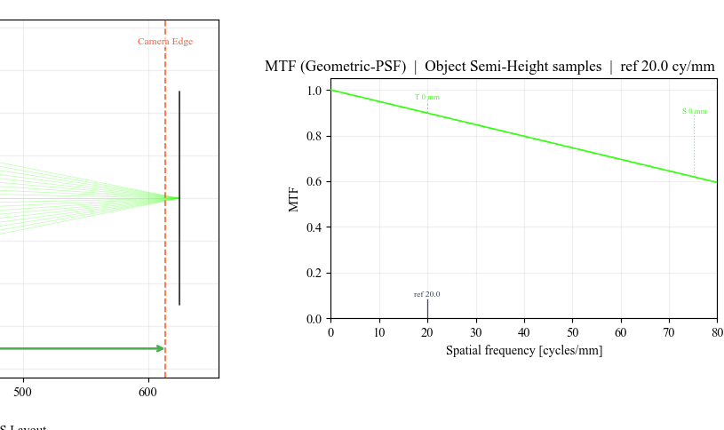
Refocused MTF AOI: the focused lens now has useful contrast at the reference spatial frequency.

Check The Wide Field

After the on-axis focus is correct, switch back to the measured wide-field setup:

Field Type  = Real Image Height
Field Value = 11.52
Field Count = 3
Spot View   = Grid

Click Spot and Update. The grid view separates the sampled field points so the user can compare center and edge behaviour.

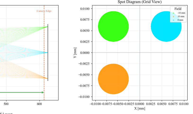
Wide-field spot AOI: after focus recovery, the center and edge field points can be compared without confusing the analysis with gross defocus.

What This Proves

This case study exercises a sequential, finite-conjugate lens workflow:

• finite object/image geometry;

• F-number aperture control;

• table editing of the image distance;

• Spot and MTF analysis modes;

• variable selection and bounds;

• deterministic best-focus optimization;

• before/after verification with regenerated screenshots.

Common Mistakes

I changed the Image row thickness.

The Image row thickness is normally zero. Change the thickness of the row before Image. In this preset that is S5 Lens Rear Datum.

I optimized a lens radius instead of sensor distance.

That changes the lens prescription. For focus recovery, mark only the final air gap / sensor distance as variable.

The wide-field plot still looks worse than the on-axis plot.

That is expected. The wide-field analysis includes off-axis field points. First remove gross defocus on-axis, then judge field performance.

Best Focus Solve and Start Optimization are both available.

Best Focus Solve is a deterministic one-variable focus search. Start Optimization is more general and is useful once you have multiple variables and multiple operands.