Working with the KrakenOS Library
This page is a faithful conversion of Section 3 of the provisional manual
(KrakenOS/Docs/USER_MANUAL_KrakenOS_Provisional.pdf, pages 10–19). It
walks a single doublet example end to end: declaring surfaces, building a
system, tracing a ray, harvesting ray state through the Raykeeper
container, and rendering the result with the Display2D / Display3D
helpers.
Python classes define an object with their attributes; instances acquire all
attributes available on the class. When creating a system, the constructor
takes a list of surfaces and a configuration object — these can be named
freely. In this section the surface list is called A, the configuration
configuration_1 and the optical system Doublet. None of those names are
required by the library.
3.1 Ray generation
Note
All rays and optical systems are drawn and traced from left to right.
KrakenOS also allows tracing right to left: surface separations are positive
left-to-right and negative otherwise. Negative Thickness values are
common with mirrors — see Example - Tel 2M Pupila in the appendix.
Import the library:
import numpy as np
import KrakenOS as Kos
In-code documentation is available through help(Kos), help(Kos.system)
and help(Kos.surf).
All optical surfaces are declared independently. Each declaration can use any subset of the parameters listed in Table 1 — surf class attributes. The five surfaces below define a simple doublet plus its object and image planes.
# Object plane
P_Obj = Kos.surf()
P_Obj.Rc = 0.0
P_Obj.Thickness = 0.1
P_Obj.Glass = "AIR"
P_Obj.Diameter = 30.0

# First face of the doublet — BK7 (crown glass, low dispersion)
L1a = Kos.surf()
L1a.Rc = 92.847
L1a.Thickness = 6.0
L1a.Glass = "BK7"
L1a.Diameter = 30.0
L1a.Axicon = 0

# Cemented interface — F2 (flint glass, high dispersion)
L1b = Kos.surf()
L1b.Rc = -30.716
L1b.Thickness = 3.0
L1b.Glass = "F2"
L1b.Diameter = 30

# Third face of the doublet
L1c = Kos.surf()
L1c.Rc = -78.19
L1c.Thickness = 97.37
L1c.Glass = "AIR"
L1c.Diameter = 30

# Image plane
P_Ima = Kos.surf()
P_Ima.Rc = 0.0
P_Ima.Thickness = 0.0
P_Ima.Glass = "AIR"
P_Ima.Diameter = 18.0
P_Ima.Name = "Image plane"
BK7 and F2 are widely used together to build achromatic doublets (Ref. 4, §11.6).
The Setup object configures the environment and, in particular, loads the
glass catalogs. Setup is defined in KrakenOS/SetupClass.py and can be
edited to include any catalog from the Cat directory. The default loads
four catalogs; UTILIDADES.AGF is required.
cat1 = (route + '/KrakenOS/Cat/SCHOTT.AGF')
cat2 = (route + '/KrakenOS/Cat/TSPM.AGF')
cat3 = (route + '/KrakenOS/Cat/INFRARED.AGF')
cat4 = (route + '/KrakenOS/Cat/UTILIDADES.AGF')
filepath = [cat1, cat2, cat3, cat4]
The default setup is loaded with:
configuration_1 = Kos.Setup()
With the surfaces and configuration in hand, the system is built from a list of surfaces and the configuration object:
A = [P_Obj, L1a, L1b, L1c, P_Ima]
configuration_1 = Kos.Setup()
Doublet = Kos.system(A, configuration_1)
Every ray has three parameters: an origin XYZ = [x1, y1, z1] and a
direction given by direction cosines LMN = [L, M, N]. A ray parallel to the
optical axis has LMN = [0, 0, 1]. In general the direction cosines are
defined by
where [x2, y2, z2] is the intersection point on the first surface.
Before ray tracing, the first-surface hit point is unknown, so direction
cosines are expressed in terms of the angle of incidence. For a ray arriving
at angle Theta from the y-axis with no x-component: L = 0,
M = sin(Theta), N = cos(Theta). The wavelength is supplied as
W in micrometres.
XYZ = [0, 14, 0]
Theta = 0.1   # field angle (degrees)
LMN = [0.0, np.sin(np.deg2rad(Theta)), -np.cos(np.deg2rad(Theta))]
W = 0.4
For rays sampled across the pupil, see the PupilCalc Tool.
The ray is traced through the doublet with:
Doublet.Trace(XYZ, LMN, W)
After Trace, the system can be queried for the result using any of the
attributes in Table 2 — system class implementations and attributes. For example Doublet.GLASS returns
the materials the ray crossed:
>>> print(Doublet.GLASS)
['BK7', 'F2', 'AIR', 'AIR']
Doublet.XYZ and Doublet.LMN return the per-surface coordinates and
direction cosines as NumPy arrays:
>>> np.shape(Doublet.XYZ)
(5, 3)
>>> np.shape(Doublet.LMN)
(4, 3)
XYZ contains one [x, y, z] per surface (object → image plane), while
LMN contains the direction cosines for each segment between surfaces.
For a five-surface system the segment chain is:
A = [P_Obj -> L1a -> L1b -> L1c -> P_Ima]
3.2 Extraction of ray information
Most analyses (spot diagrams, wavefront fits, etc.) need many rays. The
Raykeeper container stores per-ray results so the system object does
not have to. Separate containers can be created for separate fields,
wavelengths, or sources.
Rays = Kos.raykeeper(Doublet)
After each trace, call push() to commit the current ray into the
container:
Rays.push()
3.3 Generation of the optical system graph
Two helpers render a system together with the rays stored in a container:
Display2D and Display3D. Both take the system and a Raykeeper,
plus a final parameter:
Display2D(system, raykeeper, plane)—plane = 0plots the XZ plane,plane = 1plots the YZ plane.Display3D(system, raykeeper, cutout)—cutoutcontrols how surfaces are unfolded:0— full elements1— 1/4 cutout2— 1/2 cutout
For the doublet example:
Kos.Display2D(Doublet, Rays, 0)
The ray colour is derived from the wavelength used during Trace. A
0.4 µm ray appears purple, 0.6 µm appears red, and so on; wavelengths outside
the visible range are drawn in black.
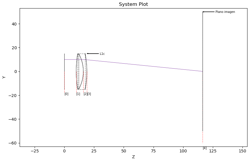
Figure 1. 2D visualization of a ray traced through a doublet.
Display2D accepts an optional fourth parameter (default 0); positive
values draw a direction arrow on every ray. The value sets the arrow size.
Kos.Display2D(Doublet, Rays, 0, 1)
For the same system in three dimensions:
Kos.Display3D(Doublet, Rays, 2)
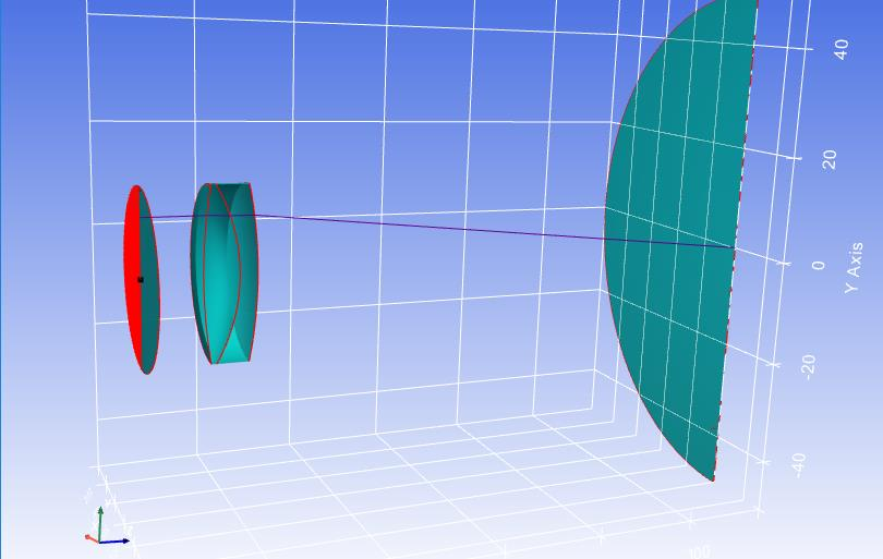
Figure 2. 3D visualization of a cross-section of the doublet and a ray.
Multiple rays can be pushed inside a loop. Code 4 traces a fan of 20 rays
parallel to the optical axis:
for y in range(-10, 10):
    XYZ = [0.0, y, 0.0]
    LMN = [0.0, 0.0, 1.0]
    W = 0.4
    Doublet.Trace(XYZ, LMN, W)
    Rays.push(Doublet)

Kos.Display3D(Doublet, Rays, 2)
Rays that do not hit any surface are recorded but not traced.
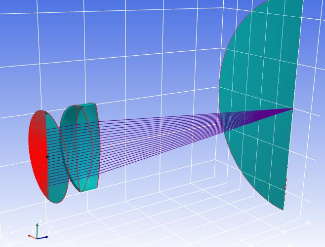
Figure 3. 3D view of the optical system with several rays.
Raykeeper introspection
A Raykeeper holds essentially the same per-ray fields exposed on the
system class, but indexed across all pushed rays — so each attribute is an
array of arrays. The number of stored rays is available as:
>>> print(Rays.nrays)
100
Rays that never hit a surface (origin or direction missed the system) are still recorded with their origin, direction and wavelength, but the rest of the per-surface fields will be empty. These are called empty rays; rays that did hit at least one surface are valid rays. The list of valid ray indices is obtained with:
>>> print(Rays.valid())
[[25] [26] [27] [28] ... [55]]
After calling valid(), a parallel set of valid_* accessors becomes
populated. These mirror the regular accessors but contain only valid rays,
with the empty rays removed (so indices shift). A separate invalid_*
namespace is also created for the empty-ray subset; only origin, direction
and wavelength can be retrieved for these.
All rays |
Valid rays |
Invalid rays |
|---|---|---|
|
|
|
|
|
|
|
|
|
|
|
|
|
|
|
|
|
|
|
|
|
|
|
|
|
|
|
|
|
|
|
|
|
|
|
|
|
|
|
|
|
|
|
|
|
|
|
|
|
|
|
|
|
|
|
|
|
|
|
|
|
|
|
|
|
|
|
|
|
|
|
|
|
|
|
|
|
|
|
|
|
|
|
|
|
|
To drop all rays from a container, either reassign the container or call
clean():
Rays.clean()