Case Study 15: Cooke Triplet Optimization From A Bad Start

Goal

This case study ports the useful workflow from Optiland Tutorial_5c_Optimization_Case_Study.ipynb into a KrakenOS UI sequence. It starts from a deliberately poor air-spaced Cooke triplet, analyzes the bad spot/MTF result, exposes the variables in the editable table, and applies a known optimized prescription so the before/after result is deterministic for a presentation.

The screenshots in this tutorial are generated from the live Tk UI with:

python -m KrakenOS.UI.capture_cooke_triplet_case_study_screenshots

The physics validator is:

python -m KrakenOS.UI.validate_cooke_triplet_case_study

Load The Poor Triplet

1. Start the UI with python -m KrakenOS.UI.layout_editor.

2. In the top menu, choose Layouts -> Starter Lenses -> Cooke Triplet Optimization Case Study.

3. Confirm the analysis controls:

   • Object Mode = Infinity;

   • Aperture = EPD;

   • EPD = 4 mm;

   • Field Type = Angle;

   • Field Value = 3 deg;

   • Field Count = 2;

   • Wavelength = 0.55 um.

The starting prescription intentionally uses very weak +/-1000 mm radii. It has the right positive-negative-positive Cooke topology, but it is not a useful image-forming lens yet.

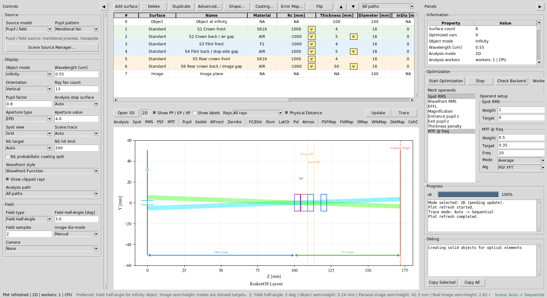
The starting Cooke-like triplet is loaded with radius and air-gap variables already marked in the table.

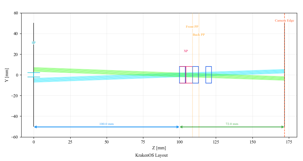
The layout has three air-spaced elements, but the surfaces are nearly flat.

Make The Bad Analysis

Click Spot and Update. The primary-wavelength spot is intentionally large. The validator checks that the starting point has more than 1 mm RMS spot radius both on-axis and at 3 deg.

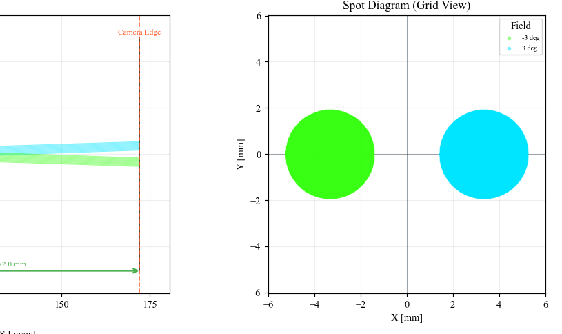
Starting Spot AOI: the nearly-flat prescription does not focus the EPD bundle.

Click MTF and Update. Use MTF @ freq = 20 cycles/mm with Alg = PSF FFT in the Optimization panel. The starting geometric MTF at this frequency is nearly zero because the image blur is too large.

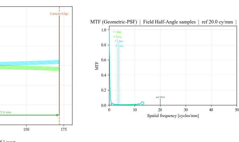
Starting MTF AOI: the poor prescription has little useful contrast at the reference spatial frequency.

Understand The Variables

The starting layout marks six radii and three air gaps for optimization:

Row	Variable	Bounds	Why it matters
S1	Radius	15, 80	Front crown power.
S2	Radius and air gap	-800, -20 and 1, 12	Back crown power and spacing to the flint.
S3	Radius	-80, -10	Front flint negative power.
S4	Radius and air gap	10, 80 and 1, 10	Back flint power and stop-side spacing.
S5	Radius	20, 800	Rear crown front power.
S6	Radius and image gap	-80, -10 and 25, 70	Rear crown back power and focus distance.

This is a true lens-design problem, not only a focus solve. The machine-vision case study changes one sensor distance. This Cooke case changes the optical prescription itself.

Apply The Optimized Prescription

For a live demo, use this deterministic prescription instead of relying on a long stochastic optimizer run. Enter these values in the table, or use the layout’s OPTIMIZED_SURFACES data as shown in KrakenOS/Examples/Examp_Cooke_Triplet_Optimization_Case_Study.py.

Row	Radius mm	Thickness mm	Glass after surface
S1 Crown front	22.01359	3.25896	SK16
S2 Crown back / air gap	-435.76044	6.00755	AIR
S3 Flint front	-22.21328	0.99997	F2
S4 Flint back / stop-side gap	20.29192	4.75041	AIR
S5 Rear crown front	79.68360	2.95208	SK16
S6 Rear crown back / image gap	-18.39533	42.20778	AIR

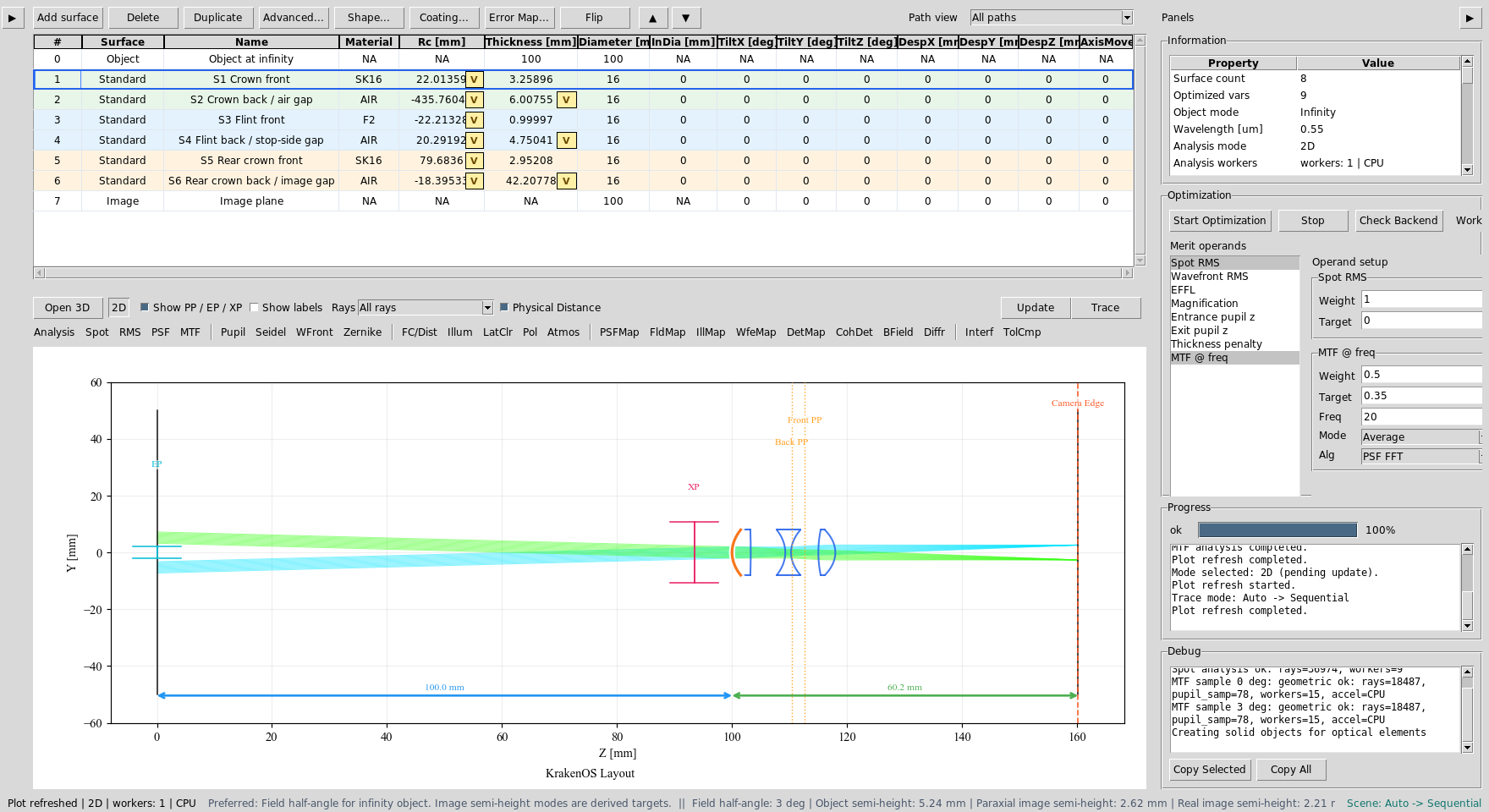
The final prescription is still the same three-element Cooke topology, but the radii and spacings now carry real optical power.

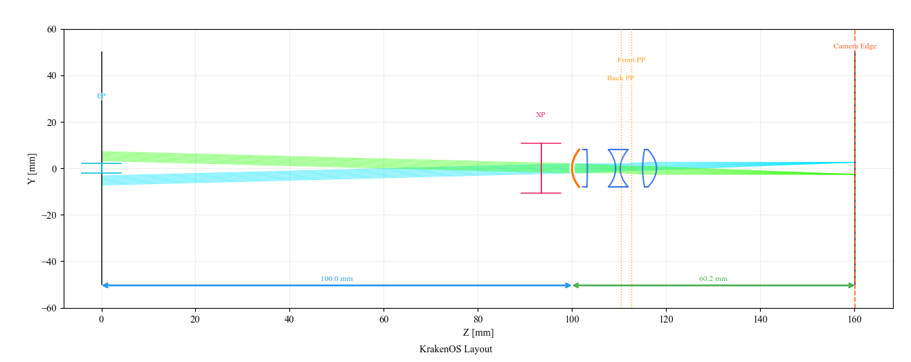
Optimized layout: the primary-wavelength rays now come to focus near the Image row.

Verify The Improvement

Click Spot and Update again. At 0.55 um, the validator checks that the optimized RMS spot is below 0.01 mm both on axis and at 3 deg.

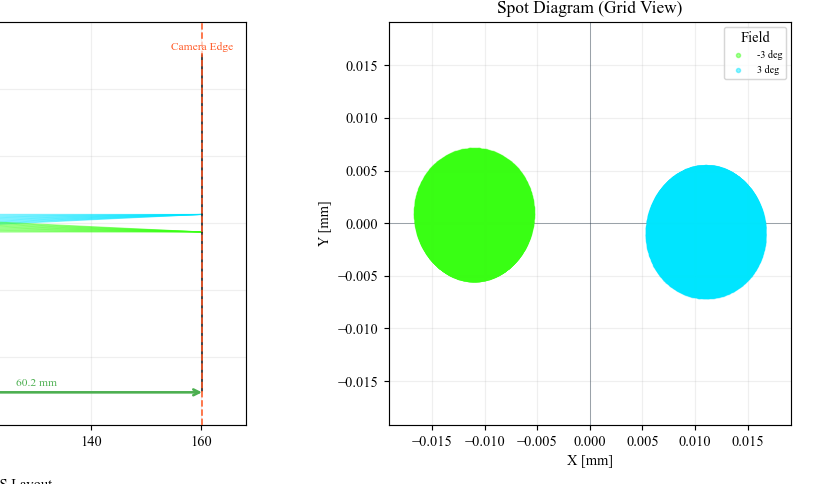
Optimized Spot AOI: the primary-wavelength spot collapses by more than 50x in mean RMS radius.

Click MTF and Update. At 20 cycles/mm the optimized primary prescription recovers useful geometric MTF, while the starting layout was nearly zero.

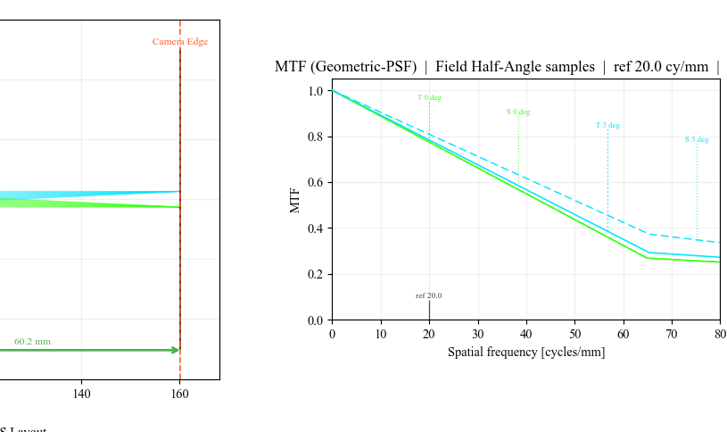
Optimized MTF AOI: the same analysis panel now shows usable contrast.

What This Proves

This case study exercises a sequential lens-design workflow:

• air-spaced multi-element prescription editing;

• real glass choices from the KrakenOS material catalog;

• six radii and three air gaps exposed as optimization variables;

• Spot and MTF analysis on a poor first design;

• deterministic optimized prescription entry;

• validator-checked primary-wavelength spot improvement.

Common Mistakes

I typed angle as lowercase angle.

Use the UI control value Angle. The KrakenOS UI maps that value to the correct field generator for off-axis rays.

I expected all three wavelengths to match Optiland exactly.

This case study validates the primary wavelength. The imported Optiland-style prescription is a teaching endpoint, not a released achromat tolerance file.

The optical diameters look generous.

They are deliberately generous in this teaching layout so the off-axis field analysis is about lens power and spacing, not mechanical vignetting.