Tracing And Ray Data

Scene-first UI model

The UI is moving toward a non-sequential scene-first architecture. The editable table is treated as a KrakenOS scene/object list. Exact sequential tracing is still first-class, but it is the axial ordered-surface special case of that scene model rather than the UI’s long-term organizing principle.

The Scene trace control therefore behaves as follows:

• Auto uses KrakenOS NsTraceLoop when the layout contains a physical source, a beam splitter, an STL optical solid, off-axis/tilted scene geometry, a non-sequential target surface, or probabilistic non-sequential coating.

• Non-Sequential Preview explicitly forces the scene trace path.

• Sequential explicitly forces the ordered-surface axial compatibility path.

• Folded Preview remains a legacy display compatibility mode for simple mirror-folded layouts.

The separate Folded reach control decides whether folded 2D display paths are allowed to define detector hits:

• Trace events keeps KrakenOS ray events authoritative. Folded display detector status, residuals, and detector surface are still written to Ray Events CSV and ray-analysis records, but they do not replace the physical terminal surface or detector-hit flag.

• Display compatibility preserves the old folded-preview behavior for layouts that intentionally use a display path as the detector reach model. This mode is explicit because it is a compatibility display workflow, not a physical non-sequential trace.

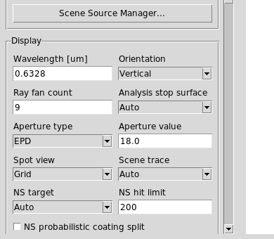
Scene trace lives in the left Display controls beside the ray count, aperture, non-sequential target, and hit-limit fields.

2D slices, 3D scenes, and CAD envelopes

The UI keeps ray generation 3D-first for scene/CAD workflows:

• The 2D layout is a display slice/projection. YZ and XZ are physical section views through the traced 3D bundle; XY is the top-view footprint. In a section view a finite-object cone appears as a triangular slice rather than a filled cone.

• Sequential Pupil / field 2D previews use one shared 3D section trace and filter it into the selected projection. If the active field span is zero, the UI disables Field Samples as NA and traces one effective on-axis field launch while preserving the requested field count in metadata.

• Ray hover/click diagnostics in the 2D plot and 3D viewers read the canonical terminal event. A missed detector/Image reports the detector surface, plane distance, radial miss, active half-aperture, local detector-plane X/Y, active detector width/height, and the original kernel terminal reason when available.

• Active detector footprints and missed-detector crosshairs are scene-target overlays, not viewer-only guesses. The 2D projector and both 3D viewers draw them from SceneTarget3D detector metadata and ray terminal events.

• The 3D inspector is not produced by revolving the 2D sketch. It retraces a source-driven 3D boundary bundle around the entrance pupil/object cone, then adapts inward to the through-going pupil envelope if the outer launch boundary is clipped by the optical train. The 3D Full Pupil toggle still requests a dense full-pupil bundle.

• Export 3D STEP uses the same source-driven 3D boundary bundle and then writes only the outer ray envelope as solid STEP tubes for mechanical review.

This separation matters for arbitrary shapes: STL/STEP solids, prisms, beam splitters, and future non-sequential components must see true world-coordinate ray directions, while the 2D view remains a readable diagnostic slice.

Sequential tracing special case

The manual’s basic workflow is:

1. Build surf objects for Object, optical surfaces, stops, mirrors, and Image.

2. Create config = Kos.Setup().

3. Create system = Kos.system(surface_list, config).

4. Trace rays with system.Trace(source_point, direction_cosines, wavelength).

5. Push traced rays into Kos.raykeeper(system).

Minimal example:

import KrakenOS as Kos

obj = Kos.surf()
obj.Thickness = 100.0
obj.Glass = "AIR"
obj.Diameter = 30.0

lens = Kos.surf()
lens.Rc = 92.847
lens.Thickness = 6.0
lens.Glass = "BK7"
lens.Diameter = 30.0

image = Kos.surf()
image.Glass = "AIR"
image.Diameter = 20.0

system = Kos.system([obj, lens, image], Kos.Setup())
rays = Kos.raykeeper(system)
system.Trace([0.0, 0.0, 0.0], [0.0, 0.0, 1.0], 0.55)
rays.push()

Non-sequential tracing

The manual introduces system.NsTrace(source_point, direction_cosines, wavelength). Current UI coverage adds:

• Auto scene tracing that resolves to NsTraceLoop for source-driven, beam-splitter, off-axis, target-surface, or coating-probability scenes

• explicit Non-Sequential Preview mode

• NsLimit

• target surface selection using TargSurf/TargSurfRest

• energy_probability for probabilistic coating branch splitting

• Beam Splitter rows that persist splitter settings, spawn deterministic reflected/transmitted child paths, and write coating tables as a fallback

• file-backed optical CAD/STL solids through native Solid_3d_stl rows; STEP/IGES vendor CAD is meshed to cached STL first, and closed meshes use the row material for non-sequential entry/exit regardless of the tilted mesh side selected by the hit chooser

• Non-Sequential Scene Graph inspection and CSV export

• Trace Path inspection and CSV export

Branches are produced by KrakenOS during NsTrace/NsTraceLoop. They are not hand-authored nodes; the UI shows them as trace diagnostics after the ray trace. Deterministic beam-splitter mode records branch identity, parent identity, power, phase metadata, and branch labels in raykeeper.

Scene source records

The UI maps the current Source panel to a first-class SceneSource3D record when no explicit scene sources are defined. For multi-source work, use Actions -> Scene Source Manager... or the Scene Source Manager... button in the Source panel. The manager edits the saved SETTINGS["scene_sources"] records, controls whether source rows appear after Object or before Object, and keeps those source rows separate from KrakenOS surf indices. Saved layouts can also declare the same records directly, for example:

SETTINGS = {
    "scene_sources": [
        {
            "source_id": "source:left",
            "name": "Left illuminator",
            "model": "Collimated disk source",
            "origin": [0.0, -10.0, 0.0],
            "direction": [0.0, 0.124, 0.992],
            "radius": 1.2,
            "ray_count": 5,
            "power": 0.6,
        },
        {
            "source_id": "source:right",
            "name": "Right illuminator",
            "model": "Collimated disk source",
            "origin": [0.0, 10.0, 0.0],
            "direction": [0.0, -0.124, 0.992],
            "radius": 1.2,
            "ray_count": 5,
            "power": 0.4,
        },
    ],
}

The source record is carried by SceneBundle.sources and exposed in the Non-Sequential Scene Graph. Physical source modes such as Collimated disk source and Gaussian beam are marked as illumination sources. The legacy Pupil / field source mode is marked as a pupil_field_reference because it is not a physical emitter independent of the Object row.

Use Actions -> Source Illumination Report after Update to audit a selected Object, aperture, splitter, detector, or Image surface. The report groups traced hits by SOURCE_ID and shows launched source rays, target-hit rays, missed/vignetted rays, hit power, power throughput, hit centroid, RMS radius, and hit span. For rays that never hit the selected target, the report also shows missed power, the dominant terminal/loss surface, and a terminal count breakdown. The report table stays compact; selecting a source row opens the full loss, power, centroid, RMS, and span details in the details pane below the table. The exported CSV includes those same loss-diagnostic fields. The Illum analysis button uses the same traced records for layouts with explicit scene sources and plots a target-surface power-density map with per-source centroids; when target rays are missed, the plot annotation includes the dominant loss terminal. This source-to-object diagnostic layer uses the same traced 3D ray data as Ray Inspector and SceneBundle, so it does not rebuild a separate illumination ray set.

For physical scene sources, Illum is normally a camera-sensor or Image-plane relative illumination plot. With target Auto, the UI therefore chooses the first traced-hit target by optical-design priority: Detector/Image, Object or Diffuse Object target, Aperture/Stop pupil plane, then any other hit surface. Use Analysis surface or the Source Illumination Report Target dropdown to override that default when you intentionally want illumination on an entrance pupil, aperture stop, exit pupil proxy, object target, or intermediate surface. The table row selection alone is not used as the Illum target, which avoids accidentally plotting illumination on a beam splitter or lens row.

Launch sampling metadata

Ray exports preserve both what the user requested and what the physical launch actually contains. This matters most for on-axis sequential layouts: a saved layout may request three field samples, but if Field Half-Angle or object height is zero, all three fields overlap. The live preview traces one effective field launch; saved rays and CSV exports record both values so the browser view does not hide either fact.

The launch metadata appears on raykeeper arrays, canonical RayEvent3D records, Ray Inspector rows, ray-analysis rows, and ray-event CSV exports:

• LAUNCH_FIELD_REQUESTED: authored field sample count.

• LAUNCH_FIELD_EFFECTIVE: distinct physical field launches after overlap collapse.

• LAUNCH_FIELD_BASIS and LAUNCH_FIELD_UNIT: angle/object-height basis.

• LAUNCH_FIELD_MIN and LAUNCH_FIELD_MAX: sampled field span.

• LAUNCH_FIELD_ACTIVE: false when the span is zero.

• LAUNCH_RAY_COUNT and LAUNCH_PUPIL_PATTERN: per-launch ray sampling.

• LAUNCH_TRACE_INTENT and LAUNCH_SAMPLING_MODE: resolved sequential or non-sequential path plus UI/saved sampling mode.

Missed detector terminals are also event-owned. Image rows are detector terminals in both sequential and non-sequential scene mode. If a non-sequential ray exits the modeled optical geometry before reaching a detector/Image surface, the scene event layer projects that terminal marker to the detector plane. It is classified as missed_image/missed_detector and remains reaches_detector=False. Ray-event and ray-analysis CSV rows preserve terminal_geometry_source=detector_miss_plane plus detector surface, projected distance, radial miss, active half-aperture, plane-normal residual, and the original kernel terminal reason. The 2D and Open 3D viewers use the same terminal status: detector hits, missed detectors, absorbed paths, escaped paths, and diagnostic stops receive distinct endpoint markers, and dense plots continue to show non-hit terminal markers even when normal detector-hit glyphs are hidden.

Actions -> Detector Aperture Report summarizes those same ray-analysis records by detector/Image surface. It reports ray/path count, unique source-ray count, detector hits, missed-detector projections, stopped/other terminals, hit and miss power, hit/miss fractions, the worst miss margin, worst local X/Y, and the dominant terminal reason. Its CSV export keeps the detector surface plus the worst-miss radial, active half-aperture, projected distance, and plane normal residual fields, so aperture clipping can be audited without reading the 2D plot by eye. The same aggregate detector hit/miss counts are written into the normal results panel after each trace, and the status bar reports a compact detector-miss warning when any detector/Image aperture is clipped. Ray Inspector top rows and CSV export also include normalized per-ray aperture status fields so each path can be read as detector hit, detector miss, detector bypass, or unrelated to a detector.

The editable table still stores KrakenOS optical surfaces. A visible Illumination Source table entry is a scene row backed by SceneSource3D, not a KrakenOS surf row. Double-click a source row to open the Scene Source Manager. Right-click the source row for direct source-row actions such as duplicate, delete, and move up/down; those actions update SETTINGS["scene_sources"] only and do not insert pseudo-surfaces. That distinction keeps source authoring from shifting detector/path surface indices.

Scene target records

The scene bundle also carries SceneTarget3D records. These records make Object, Object Target, Diffuse Object, Aperture, Image/detector, and explicitly selected non-sequential target rows visible as object/detector scene entities without adding or reordering KrakenOS surf indices. Object and Image rows remain reference/detector targets by default; they do not become movable ScenePlacement3D handle records, and old placement metadata on those reference rows is ignored by the 3D handle layer.

Each target record stores:

• row index and trace-surface index;

• target role, such as object_reference, object_target, aperture, detector, or analysis_target;

• world center, normal, and tangent vectors used by display/analysis tooling;

• detector active area, detector bins, and pixel pitch when detector metadata is present;

• whether the record is a detector, an object/reference, or the active TargSurf selection.

Actions -> Non-Sequential Scene Graph exposes these records under Scene targets. Use Edit Target in that window to update target identity without creating a UI-only abstraction. The editor stores target role metadata on the surface row, writes detector active area/bins/pixel pitch through the same detector metadata used by detector analyses, and can set or clear the active non-sequential TargSurf selection.

Choosing Detector marks the selected non-Object row as a detector target. Choosing Object Target, Diffuse Object, or Aperture applies the same surface-type defaults used by the editable table, so KrakenOS tracing still receives ordinary prescription rows. Choosing Analysis Target keeps the surface type unchanged but persists a scene-target role for diagnostics and future target-aware analysis.

Possible next scene workflows

White-light triangular-prism dispersion is compatible with the North Star. It should be implemented as a wavelength-sampled physical source, not a 2D color overlay. The trace should launch the same beam over a wavelength list, let the glass catalog produce wavelength-dependent refractive indices, and store each ray’s wavelength in canonical events. The 2D and 3D renderers can then color the same traced rays by wavelength and a detector target can report the chromatic spot/rainbow footprint.

Direct placement of imported STEP optical components in the 3D plot is also compatible with the current architecture. STEP/IGES already converts to cached STL for tracing, and CAD/STL faces already carry placement and optical-role metadata. Rows can now also carry ScenePlacement metadata for grid visibility, linear snap spacing, angular snap step, and placement anchor intent. SceneBundle exposes those records as ScenePlacement3D objects, and the Non-Sequential Scene Graph exports them beside sources, targets, volumes, and boundary faces. Open 3D renders a placement grid from the selected or first visible placement record and shows the active snap/grid values in a VTK overlay. The visible translation handles move the selected row along global X/Y/Z by ScenePlacement snap spacing when snap is enabled, or by the grid spacing when snap is off. Each move writes DespX/Y/Z plus placement metadata through the normal row history/table path. Rotation handles rotate the selected row around global X/Y/Z by ScenePlacement.snap_deg when snap is enabled, or by a coarse 15 degree step when snap is off, and write TiltX/Y/Z through the same row history/table path. Dragging a placement handle accumulates screen motion and applies repeated snap steps through the same row-backed services; clicking without dragging remains the precise one-step fallback. A full 3D placement tool should still add richer face/axis picking, but those controls must persist back to row pose plus ScenePlacement and optical-solid metadata. The same scene state must drive the 2D projection, 3D display, tracing, scene graph diagnostics, and CSV export.

Source orientation uses direction cosines L/M/N in global X/Y/Z axes. In the usual YZ 2D layout, +Z is horizontal to the right and Y is vertical on the page. Use the Source panel Direction preset dropdown for the common cases:

Preset	LMN	Meaning in YZ layout
Horizontal +Z (right)	0, 0, 1	Launch left-to-right along the optical table axis.
Horizontal -Z (left)	0, 0, -1	Launch right-to-left.
Vertical +Y (up)	0, 1, 0	Launch upward on the YZ plot.
Vertical -Y (down)	0, -1, 0	Launch downward from a top port.

The older Display orientation control only changes the 2D plot/view orientation. It does not rotate a physical source.

SceneBundle.scene_row_mapping carries the bridge for that visible table. It maps scene rows to current table rows and KrakenOS trace surfaces. For a reset scene with one physical source, the default scene-row order is:

Scene row	Kind	Trace surface
0 / S0 Object	Surface	0
1 / Src1 Source 1	Illumination source	None
2 / S1 Image	Surface	1

This lets the UI later show Object + Illumination Source + Image without changing the trace indices consumed by raykeeper, detector paths, and analysis tools.

Actions -> Non-Sequential Scene Graph exposes the same mapping today. The tree has a Scene row order node and columns for scene row, current table row, trace surface, and source ID. Use it to confirm whether a source is a physical scene emitter or an optical surface before relying on detector/path indices.

For illumination-first layouts, set scene_row_order="before_object" in layout SETTINGS. The future scene-row order then becomes Src1 Source 1, S0 Object, S1 Image while trace surfaces remain 0 and 1. This is intended for source/object split systems where the user thinks of placing a lamp or laser first, then the object, then imaging optics.

For source/object split fixtures that need a return path today, use the table surface type Object Target. It is intentionally semantic: the UI presents it as the object location, while the current tracing backend maps it to a specular reflective proxy. This avoids labeling the object as a normal Mirror in the workflow.

Use Diffuse Object when the object should scatter instead of returning one specular proxy ray. Its DiffuseScatter metadata uses the built-in Lambertian, Oren-Nayar, Cosine Lobe, or optional pySCATMECH backend: a hit spawns deterministic child branches named scatterNN and records their powers in BRANCH_POWER. For imaging fixtures, set target_surface in that metadata to a pupil, lens, detector, beam splitter return aperture, or Image surface; the core then importance-samples that target with approximate model-weighted solid-angle weights instead of wasting most rays outside the useful camera path.

For detector-plane coherence analysis, CohDet now supports grouping modes: All rays coherent, By source ray, By source, and Incoherent power only. By source ray is the practical default for interferometers and source bundles because complementary branches from one launched source ray still interfere, while independent launches add as intensities instead of one global field.

The same detector-bin machinery now exposes branch-code self terms and complementary branch-pair interference terms on the detector grid. Detector- bearing interferometer layouts can therefore let Interf reuse the coherent detector accumulation when the detector sampling is dense enough; sparse single-ray presets still fall back to the analytic path-average diagnostic. The Diffr analysis then takes the same coherent detector field and computes a vector Fraunhofer/angular-spectrum FFT, with coherent groups handled according to the selected coherence mode. The detector-bin stability validator checks that changing the detector grid does not silently change the traced sample set, branch-code set, coherence grouping, incoherent power accounting, all-rays Jones-vector intensity, or unitary FFT power conservation.

Regression check:

python -m KrakenOS.UI.validate_object_target_surface
python -m KrakenOS.UI.validate_diffuse_object_scatter
python -m KrakenOS.UI.validate_diffuse_object_cosine_lobe
python -m KrakenOS.UI.validate_diffuse_object_oren_nayar
python -m KrakenOS.UI.validate_diffuse_object_pyscatmech
python -m KrakenOS.UI.validate_coherent_detector_modes
python -m KrakenOS.UI.validate_interferogram_detector_accumulation
python -m KrakenOS.UI.validate_diffraction_detector
python -m KrakenOS.UI.validate_detector_sampling_stability
python -m KrakenOS.UI.validate_detector_aperture_analysis

Each traced ray also carries source identity metadata:

• SOURCE_ID: stable source key such as source:0 or source:left

• SOURCE_NAME: user-facing source name such as Source 1 or Left illuminator

• SOURCE_ROLE: illumination or pupil_field_reference

• SOURCE_MODEL, SOURCE_XYZ, SOURCE_LMN, SOURCE_POWER, SOURCE_WEIGHT, and SOURCE_WAVELENGTH: launch model and launch state

Validate this plumbing with:

python -m KrakenOS.UI.validate_scene_sources
python -m KrakenOS.UI.validate_multi_scene_sources
python -m KrakenOS.UI.validate_scene_row_mapping
python -m KrakenOS.UI.validate_scene_source_row_contract
python -m KrakenOS.UI.validate_gaussian_branch_frames

validate_scene_row_mapping also checks row-backed 3D placement state. The coverage includes ScenePlacement snap/grid metadata, Open 3D translate and rotate handle services, and the Snap Row->Target service that moves one row or face onto another row or face while preserving the solved target-surface constraint in row metadata. It also covers Orient Row->Target, which solves row TiltX/Y/Z so a selected row or face normal aligns to another row or face normal and stores the solved target-normal constraint in the same metadata. The same validator now checks vector-backed orientation for Orient Row->Ray: a selected row or face normal can be aligned to an arbitrary traced ray direction, with the target vector, ray index, and residual angle error persisted as ScenePlacement metadata. It also checks Orient Row->Source and Orient Row->Path services, which persist source-vector and Path-frame constraints, including source origin/direction, branch path, nearest target point, and residual angle error. The validator also covers immediate local-axis and explicit scene-source orientation: Orient Row->CAD Axis records the selected row-local axis vector, and Orient Row->Scene Source records the explicit source id/name, origin, direction, model, ray count, and residual angle error. Named normal target coverage is included as well: the validator checks Preview Normal for detector/object targets, verifies that preview does not mutate row pose, and verifies that Orient Row->Normal records detector_normal or object_normal metadata with target row/id/name/role, target point, target normal, and residual angle error. validate_layout_plot_controller also checks detector-miss terminal projection so escaped rays that intersect the detector plane outside the active aperture are displayed and exported as misses instead of arbitrary short terminal segments.

Optical STL prism check

For a prism STL rotated into the classic dispersion pose, the first STL hit should not report n=1 -> 1. A BK7 prism entry should report approximately n=1 -> 1.518 at 0.55 um and the outgoing direction should bend toward the prism base. Run the regression check with:

python -m KrakenOS.UI.validate_stl_prism_media

Face-role metadata check

After changing the CAD/STL optical face workflow, run:

python -m KrakenOS.UI.validate_optical_solid_face_roles

This clusters the bundled prism STL into planar candidates, verifies automatic input/output role assignment, checks that candidates expose triangle meshes for 3D click-picking, checks beam-splitter split-ratio persistence, and confirms that saved OpticalSolidFaces metadata survives the advanced attribute parser. It also verifies that assigned face roles transform into finite unit-normal markers for the 3D inspector and CAD/STL placement preview.

Face-anchor snap-to-ray check

After changing the CAD/STL placement workflow, run:

python -m KrakenOS.UI.validate_optical_solid_snap_to_ray

This validates the first Phase 7 prism/CAD improvement: when a file-backed optical solid has saved face metadata, Center Row->Ray prefers the best assigned optical-face anchor instead of the generic row origin. The regression uses the bundled prism STL and checks that a designated transmitted left face is selected and snapped onto the chosen axial ray.

Face-fit placement check

After changing face-driven CAD/STL placement, run:

python -m KrakenOS.UI.validate_optical_solid_face_fit

This validates the next Phase 7 slice: the placement helper can choose a saved anchor face, align that face normal to the optical axis, center the anchor on the row plane, and apply a simple side-label-based roll constraint when a compatible guide face is available.

Path-frame face-fit check

After changing traced ray/path-driven CAD/STL placement, run:

python -m KrakenOS.UI.validate_optical_solid_path_fit

This validates the next placement step: the same face-fit solver can use the currently selected traced ray or current Path-view frame as the target direction and target point. The regression loads a traced beam-splitter layout, attaches a controlled branch-ray bundle, solves a prism face onto that selected ray, repeats the solve against the current Path dropdown frame, and verifies that Save Roles stores row-relative decenter correctly when the CAD/STL row is not at Z=0. It also covers the table workflow where a newly inserted CAD/STL row is snapped to the outgoing traced segment of the previous table surface instead of an earlier, merely closer ray segment.

Virtual internal plane check

After changing cube-style virtual internal optical-plane authoring, run:

python -m KrakenOS.UI.validate_optical_solid_virtual_plane

This validates the next CAD authoring slice: a labeled cube-like optical solid can derive a saved internal beam-splitter diagonal, preserve it in OpticalSolidFaces, and transform that plane into world coordinates for 3D preview and placement.

Optical-solid hit-sequence check

After changing how traced CAD/STL hits map back onto assigned optical faces, run:

python -m KrakenOS.UI.validate_optical_solid_hit_sequence

This validates the next Phase 7 CAD authoring slice: traced hits on an optical solid can be classified back to the saved face-role metadata, and crossings of saved virtual internal planes can be inserted into the ordered hit sequence. The regression uses a real traced prism STL chief ray and checks the expected Left -> Right -> Down -> Left face sequence. It also compares the same hit order against canonical ray-event records and scene graph boundary-face records so closed-solid media state, runtime mesh face ids, TIR/refraction labels, and face-role metadata stay synchronized. The same validator then adds a synthetic cube-beam-splitter crossing to confirm the virtual splitter plane appears in the correct position between the entry and exit faces.

Raykeeper data

The manual lists the raykeeper arrays as the persistent version of system ray state. The UI Ray Inspector exposes the same categories:

Category	Manual arrays	UI data product
Surface path	SURFACE, NAME, GLASS	Ray Inspector hit table and CSV.
Coordinates	XYZ, S_XYZ, T_XYZ, OST_XYZ	Ray Inspector XYZ columns and 2D/3D ray picking.
Direction cosines	S_LMN, LMN, R_LMN	Ray Inspector incoming/outgoing direction columns plus the surface-normal columns in Inspect Ray / Surface Physics.
Gaussian branch frame	Derived from LMN, R_LMN, and S_LMN	Ray Inspector and Trace Path Inspector GB K, GB T, GB S, and Inc [deg] columns. GB K is the outgoing local propagation axis, GB T is tangential, and GB S is sagittal.
Optical path	DISTANCE, OP, TOP, TOP_S	Ray Inspector distance/OP totals and CSV.
Index and material	N0, N1, ALPHA, BULK_TRANS	Ray Inspector refractive index and transmission fields.
Gratings	G_LMN, ORDER, GRATING_D	Grating rows plus inspector output.
Polarization	RP, RS, TP, TS, TTBE, TT	Ray Inspector and coating/polarization report.
Interaction bookkeeping	INTERACTION_TYPE, INTERACTION_MODEL, INTERACTION_TARGET_SURFACE, INTERACTION_IN_POWER, INTERACTION_COEFF, INTERACTION_OUT_POWER, INTERACTION_LOSS_POWER, INTERACTION_BULK	Actions -> Inspect Ray / Surface Physics and Trace Path Inspector hit tables and CSV export.
Source identity	SOURCE_ID, SOURCE_NAME, SOURCE_ROLE, SOURCE_MODEL, SOURCE_XYZ, SOURCE_LMN, SOURCE_POWER, SOURCE_WEIGHT, SOURCE_WAVELENGTH	Scene source records, Ray Inspector source columns, and branch analysis.
Launch sampling	LAUNCH_FIELD_REQUESTED, LAUNCH_FIELD_EFFECTIVE, LAUNCH_FIELD_BASIS, LAUNCH_FIELD_UNIT, LAUNCH_FIELD_MIN, LAUNCH_FIELD_MAX, LAUNCH_FIELD_ACTIVE, LAUNCH_RAY_COUNT, LAUNCH_PUPIL_PATTERN, LAUNCH_TRACE_INTENT, LAUNCH_SAMPLING_MODE	Canonical RayEvent3D records, Ray Inspector, ray-analysis CSV, and ray-event CSV.

Inspect Ray / Surface Physics

Use Actions -> Inspect Ray / Surface Physics after Update to inspect one hit at a time. The hit table now exposes:

• Incoming direction, outgoing direction, and surface normal for each hit.

• Interaction type/model plus any guided target surface for scatter/splitter paths.

• Per-hit power accounting: input power, coefficient, output power, loss, and bulk term.

This is the quickest way to confirm whether a hit reflected, refracted, transmitted, scattered, or split as expected before moving on to detector or illumination analysis.

To validate the interaction bookkeeping end-to-end, run:

python -m KrakenOS.UI.validate_interaction_accounting

Multicore and batch tracing

The manual appendix includes a multicore example. The current UI uses batch tracing where safe, scalar tracing where required by custom surface behavior, and background workers for heavier analyses and optimization.