Beam Splitters

The UI now has a Beam Splitter surface type. It is a first UI/core bridge for splitters with deterministic non-sequential child paths.

Terminology

The visible UI uses one workflow term: Path. A path is the editable physical ray segment between optical graph nodes such as source, beam splitter, mirror, another beam splitter, or detector. This is the term used by plot labels, table badges, Path view, right-click assignment menus, and detector placement helpers.

KrakenOS internals still use branch field names for traced child rays: BRANCH_ID, PARENT_BRANCH_ID, BRANCH_PATH, and related CSV columns. Those are trace metadata names, not the user-facing grouping term. Saved UI metadata also keeps legacy-compatible keys such as arm_role, leg_id, branch_selector, and arm_distance; the editor displays and documents them as path role, path ID, split selector, and path distance.

Current capability

Beam Splitter rows store a BeamSplitter metadata dictionary. Fixed deterministic mode automatically writes a KrakenOS Coating = [R, A, W, THETA] fallback table. Deterministic coating table mode instead preserves and reads the row coating table at the traced wavelength and incidence angle. Deterministic Fresnel P/S mode uses KrakenOS core Fresnel P and S coefficients with a scalar P-polarization fraction and stores normalized local Jones amplitudes plus a global branch polarization vector. All deterministic modes can also apply simple transmitted/reflected S-vs-P retardance controls through transmit_s_phase_deg and reflect_s_phase_deg. With Non-Sequential Preview, deterministic modes spawn both child paths from each splitter hit:

• transmitted path with T = 1 - R - A

• reflected path with R

• branch metadata in raykeeper.BRANCH_ID, PARENT_BRANCH_ID, BRANCH_POWER, BRANCH_PHASE, BRANCH_LABEL, and BRANCH_PATH

• branch polarization metadata in BRANCH_JONES_P, BRANCH_JONES_S, and BRANCH_POLARIZATION_XYZ

• launch metadata in SOURCE_RAY, SOURCE_XYZ, SOURCE_LMN, SOURCE_MODEL, SOURCE_POWER, SOURCE_WEIGHT, SOURCE_WAVELENGTH, LAUNCH_FIELD_REQUESTED, LAUNCH_FIELD_EFFECTIVE, LAUNCH_TRACE_INTENT, and LAUNCH_SAMPLING_MODE

Monte Carlo coating split remains available for legacy one-path stochastic coating experiments. Use a deterministic mode for normal beam-splitter design.

Split modes

Mode	Path power source	Use when
Deterministic paths	Reflectance R and Absorption A in the beam-splitter settings. Transmission is 1 - R - A.	You want an ideal/fixed ratio such as 50/50 independent of angle and wavelength.
Deterministic coating table	Interpolated row Coating = [R, A, W, THETA] at the current trace wavelength and incidence angle. The fixed R/A fields are only fallback values if no valid coating table exists.	You want path power to follow coating data from the Coating dialog or a saved Python layout.
Deterministic Fresnel P/S	KrakenOS Fresnel RP, RS, TP, and TS coefficients at the splitter hit, weighted by Polarization P fraction. 1 is pure P, 0 is pure S, and 0.5 is an equal P/S input. S phase [deg] sets the input relative Jones phase of the S component. T S-ret [deg] and R S-ret [deg] add output S phase relative to P on the transmitted and reflected child paths.	You want angle/material-dependent dielectric or metal Fresnel path power plus detector coherent sums that include P/S polarization overlap.
Monte Carlo coating split	The legacy stochastic one-path coating probability.	You are reproducing old non-sequential coating experiments rather than designing both splitter paths at once.

UI workflow

1. Load Common Optical Layout -> Beam Splitter 50/50 Example.

2. Select the splitter row, or change an ordinary row’s surface type to Beam Splitter.

3. Right-click the row and choose Beam splitter settings....

4. Set Reflectance R and Absorption A. Transmission is T = 1 - R - A. If you select Deterministic coating table, open Coating... on the same row and enter a valid [R, A, W, THETA] table; Reflectance R and Absorption A become fallback values.

5. If you select Deterministic Fresnel P/S, set P fraction to 1 for pure P polarization, 0 for pure S polarization, or 0.5 for equal P/S amplitude. Set S phase [deg] if the source is elliptical or circular in the splitter’s local P/S basis. Set T S-ret [deg] or R S-ret [deg] to model a simple coating phase delay of S relative to P on the corresponding output path. The fixed Reflectance R and Absorption A values are fallback values if Fresnel inputs are unavailable.

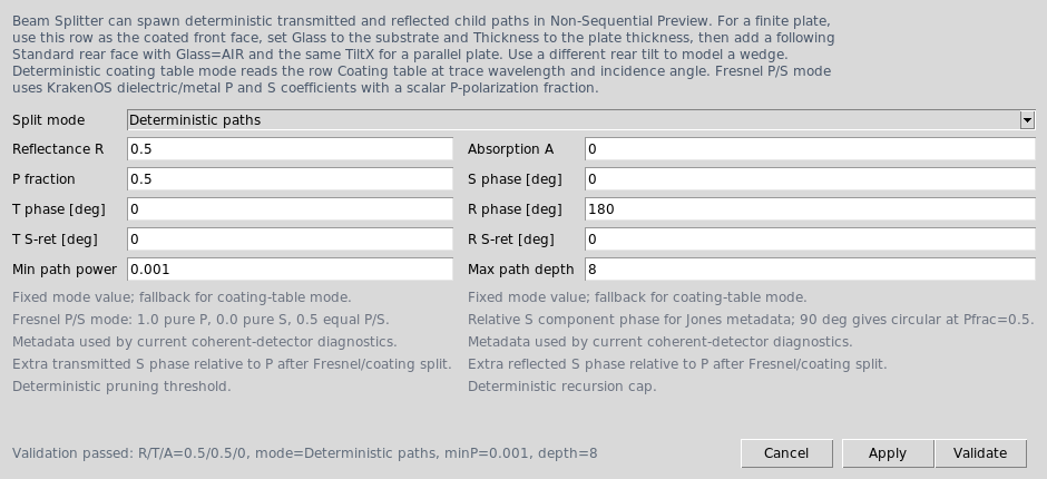
The beam-splitter settings dialog controls deterministic path splitting, Fresnel P/S input, output retardance, and recursion limits.

6. Use a physical source such as Collimated disk source or Gaussian beam. With a physical source, beam splitter, off-axis geometry, target surface, or non-sequential coating-probability request, Auto scene trace resolves to Non-Sequential Preview; explicit Non-Sequential Preview is still available. Source X/Y/Z set the physical launch origin, and Source L/M/N set the normalized chief-ray direction. In this mode the Object row is a scene/reference datum, not the source of the launched rays.

7. Leave NS probabilistic coating split off for deterministic splitters.

8. For a finite plate, set the splitter row Glass to the substrate, set Thickness to the plate thickness, and add a following Standard row with Glass=AIR as the rear face. In the editable UI table, use the same rear TiltX as the front face for a parallel plate; use a different rear tilt to model a wedge.

9. Right-click any grouped element and use Element settings... or Path role to mark it as Common, Transmit, Reflect, or Detector. The first # cell shows a compact path-role badge such as T or R on the first row of the element.

10. Right-click a Beam Splitter row and choose Add detector to transmitted path... or Add detector to reflected path... to insert a detector plane at a distance measured along that central path.

11. Use the table toolbar Path view dropdown when you want to show the full layout or isolate one discovered path. Row numbers remain KrakenOS surface indices even when the table is filtered.

12. Click Update and inspect paths with Actions -> Ray Inspector, Actions -> Trace Path Inspector, and Actions -> Non-Sequential Scene Graph.

Path view filters the table and plot to the full layout or one traced path after Update discovers deterministic splitter paths.

The Beam Splitter 50/50 Example uses an exact-count collimated disk source. Each launched source ray creates transmitted and reflected trace records, so the Ray Inspector can show the source-ray index, path power, and launch metadata for each child path.

BRANCH_LABEL is the local leaf label, such as transmit or reflect. BRANCH_PATH is the cumulative traced splitter path, for example S1:BS1/transmit -> S4:BS2/reflect. Use BRANCH_PATH for cascaded splitters, return paths, and future recombination diagnostics.

For small ray counts, the collimated and Gaussian physical source previews use equal-spaced meridional samples inside the requested radius. The outer preview rays are kept conservatively inside the source edge, which avoids accidental path loss on tilted finite plates whose projected clear aperture is smaller than their nominal diameter. Larger source bundles switch to deterministic golden-angle disk filling so the 3-D source footprint is represented.

Ray count is the number of launched source rays, not the final number of drawn paths. A deterministic 50/50 splitter therefore produces up to 2 * ray_count displayed child paths: one transmitted and one reflected path per source ray. If a finite aperture clips one path, the Ray Inspector will show fewer child records for that path.

Path workflow tutorial

Use this workflow when you want to build a first two-path splitter layout without manually calculating the reflected detector pose.

1. Start the editor and press Reset if the table is not empty.

2. Load Common Optical Layout -> Beam Splitter 50/50 Example.

3. In Source Field, choose Collimated disk source for ray-bundle debugging or Gaussian beam for a laser-style source.

4. Set Ray count to the number of launched source rays you want. With a deterministic splitter, each unclipped input ray can produce one transmitted child and one reflected child.

5. Right-click the 50/50 coated front face row and choose Beam splitter settings.... Confirm Reflectance R = 0.5, Absorption A = 0, and deterministic splitting.

6. Right-click the same front-face row and choose Add component to transmitted path.... Select Detector plane, Aperture stop, Thin lens, Refractive surface, Mirror, or Object Target, enter the distance from the splitter and clear diameter, then press Insert. The older Add detector to transmitted path... shortcut opens the same dialog with Detector plane preselected.

7. Right-click the front-face row again and choose Add component to reflected path... or Add detector to reflected path.... Enter the reflected-path distance and component parameters, then press Insert.

8. Click Update. The 2-D/3-D plots should show source rays forking into the transmitted and reflected paths, subject to finite-aperture clipping. The 2-D plot labels discovered paths directly on representative rays as Path 1, Path 2, and so on. Use the Show labels checkbox above the 2-D plot to hide these labels when dense sources, such as imported LED ray files, generate many sampled ray histories. Use the adjacent Rays selector to switch between every traced ray, detector-hit rays, and representative non-primary beam-splitter paths.

9. Use Path view -> Path 1: ... style entries to filter the table and 2-D plot to one discovered path.

10. For a nested/cascaded splitter path, choose the traced Path view entry and use Actions -> Add Component to Current Path View.... The helper derives the component frame from the latest traced BRANCH_PATH segment instead of assuming the nominal global +Z input ray.

11. To insert a real Edmund/Thorlabs catalog lens on a traced path, keep the traced Path view selected and use Insert -> Stock Lens to Current Path View... or Actions -> Add Stock Lens to Current Path View.... The catalog importer adds a Path distance field and writes the chosen stock lens as one rigid multi-row element on that path frame. The same dialog also exposes local X/Y offsets and local X/Y/Z tilts, so the block can be nudged or tipped in the selected branch frame without calculating global table values.

12. Open Actions -> Ray Inspector. The path rows should show matching source_ray values, split labels such as transmit and reflect, and path powers derived from the splitter settings.

The path-component helper inserts a native KrakenOS row before Image and tags it with Element metadata. The component mapping is:

Dialog component	Table row created	Parameter meaning
Detector plane	Standard / AIR	No extra parameter. Tagged as arm_role=Detector for detector analyses.
Aperture stop	Aperture / AIR	No extra parameter. Diameter is the clear stop.
Thin lens	Thin Lens / AIR	Focal length in millimetres, stored in the table Rc column because the runtime builder maps Rc to KrakenOS Thin_Lens.
Refractive surface	Standard / selected glass	Radius of curvature in millimetres. Add a second surface if you need a finite-thickness singlet.
Mirror	Mirror / MIRROR	Mirror radius in millimetres; 0 means flat.
Object Target	Object Target / internal MIRROR proxy	Semantic object-location row for source/object split fixtures. It returns one specular proxy ray.
Diffuse Object	Diffuse Object / internal MIRROR with DiffuseScatter metadata	Lambertian object-scatter row. It spawns deterministic scatterNN branches in non-sequential tracing.

Example metadata for a reflected-path detector row:

{
    "element_id": "Reflect_detector",
    "element_name": "Reflect detector",
    "arm_role": "Detector",
    "parent_splitter": "Splitter",
    "branch_selector": "reflect",
    "branch_path": "",
    "arm_distance": 60.0,
    "local_decenter_x": 2.5,
    "local_decenter_y": -1.25,
    "local_tilt_x": 4.0,
    "local_tilt_y": -2.0,
    "local_tilt_z": 7.0,
    "path_component_type": "Detector plane",
}

local_decenter_x and local_decenter_y are transverse offsets in the selected branch frame. local_tilt_x, local_tilt_y, and local_tilt_z are applied relative to the branch-aligned surface frame before the UI writes global TiltX/Y/Z values to the table.

For splitter-row context-menu placement, the helper uses the selected splitter surface normal and the nominal incoming global +Z ray. This is correct for the supplied straight-input beam-splitter examples. For nested/cascaded paths, first click Update, choose a traced Path view entry, then use Actions -> Add Component to Current Path View.... That helper derives the origin and direction from the latest traced BRANCH_PATH ray segment, places the component at the requested distance from the last splitter hit, and saves exact branch_path metadata such as:

{
    "element_id": "Path_TR_detector",
    "element_name": "Path TR detector",
    "arm_role": "Detector",
    "parent_splitter": "BS1 transmit -> BS2 reflect",
    "branch_selector": "reflect",
    "branch_path": "S1:BS1/transmit -> S4:BS2/reflect",
    "arm_distance": 20.0,
    "path_component_type": "Detector plane",
    "path_frame_source": "traced_branch_path",
}

The traced-path helper covers arbitrary traced splitter-to-splitter or return paths after Update. The stock-lens path importer uses the same traced frame and keeps every imported catalog surface in one element block. It preserves the catalog row spacing through path_component_axial_offset metadata and writes global TiltX/Y/Z plus DespX/Y/Z values for each row so the block sits on the selected path without manually calculating pose.

Example metadata added to every stock-lens row placed on a traced path:

{
    "element_id": "Path_TT_08068",
    "element_name": "Path TT 08068",
    "arm_role": "Transmit",
    "branch_selector": "transmit",
    "branch_path": "S4:BS1/transmit -> S8:BS2/transmit",
    "arm_distance": 35.0,
    "path_component_type": "Stock lens block",
    "path_component_part": "08068",
    "path_component_row_count": 2,
    "path_component_axial_offset": 3.21,
    "local_decenter_x": 1.5,
    "local_decenter_y": -2.0,
    "local_tilt_x": 3.0,
    "local_tilt_y": 0.5,
    "local_tilt_z": -1.0,
    "path_frame_source": "traced_branch_path",
}

To adjust a placed path element later, select the element block, right-click, and choose Geometry -> Edit path-local pose.... The dialog edits Path distance, Local X/Y offset, and Local tilt X/Y/Z in the same branch-local frame used at insertion time, then rewrites the global TiltX/Y/Z and DespX/Y/Z table cells. For traced BRANCH_PATH rows, click Update first so the latest traced segment is available. The same repose helper is also used when Element settings... is applied to a placed path element, so saved path-component metadata is not lost.

When any numbered Path view is active, the editable table presents those same path-local fields directly for path-placed components:

Table column in Path view	Meaning for path-placed rows
Local TiltX/Y/Z	Surface tilt relative to the selected branch frame.
Local X and Local Y	Transverse decenter in the selected branch frame.
Path Dist	Longitudinal distance along the selected branch from the splitter or traced path-frame origin.

Path view -> All paths switches back to the canonical global Tilt and Desp columns. Only rows inserted by the path-component or path stock-lens helpers use the virtual local columns; manually grouped/assigned rows keep their normal global table values.

The Python example KrakenOS/Examples/Examp_Phase6_Path_Component_Placement.py shows the same helper calculations headlessly and prints the generated Tilt/Decenter rows.

Two-path doublet example

Load Common Optical Layout -> Beam Splitter Two Path Doublets for a complete example where one cemented doublet is placed after the transmitted path and a second cemented doublet is placed after the reflected path.

The row structure is:

1. Object is a global reference plane; the Source panel launches the physical source bundle.

2. Splitter rows model the tilted 3 mm BK7 50/50 plate.

3. Transmit doublet rows are centered on the transmitted chief ray after the plate exit offset.

4. Transmit path detector receives the transmitted path after that doublet.

5. Reflect doublet rows are tilted so their local +Z axis follows the reflected +Y path.

6. Reflect path detector receives the reflected path after that doublet.

7. Image remains a global diagnostic surface at the end of the canonical KrakenOS table.

The important pattern is the saved Element metadata. The transmitted doublet rows use:

{
    "element_id": "TX_DBL",
    "element_name": "Transmit doublet",
    "arm_role": "Transmit",
    "parent_splitter": "BS1",
    "branch_selector": "transmit",
    "arm_distance": 33.0,
}

The reflected doublet rows use the same pattern with arm_role="Reflect" and branch_selector="reflect". The reflected surfaces also use tilt_x=-90 plus global decenter values so their physical surface normals point along the reflected path. KrakenOS still traces against those physical surface poses; the metadata is for path labels, focus selection, grouping, and future path-workbench editing.

Manual path assignment

Use manual path assignment when you add or import components surface-by-surface:

1. Select contiguous rows that form one optical component.

2. Right-click the first # cell and choose Group as Element if the rows are not already grouped.

3. Right-click the grouped element and choose Path role -> Assign to Transmit path or Path role -> Assign to Reflect path.

4. Open Element settings... if you need to set the parent splitter, split selector, path distance, or path-local offsets for documentation and future analysis.

5. Use Move Up or Move Down to reorder the element within the same path.

The path assignment metadata does not force ray routing. KrakenOS still traces against actual geometry. The metadata is used by the editor for grouping, selection, row movement, saved-layout documentation, and path-aware analysis. The table currently focuses path rows by selecting and scrolling to them rather than hiding all other rows. This preserves the KrakenOS surface-index mapping while the virtual path-workbench table remains a metadata layer on top of the canonical KrakenOS surface list.

Path Workbench workflow

The intended beam-splitter workflow is:

1. Author the common path first: source, object/reference, pre-splitter optics, and the first splitter.

2. Click Update. The editor traces deterministic paths and discovers path families.

3. The 2-D plot labels discovered paths as Path 1, Path 2, Path 3, and so on, with each label anchored to a representative ray. For nested splitters, the stable internal identity remains a BRANCH_PATH value such as BS1/transmit -> BS2/reflect. Show labels controls whether these plot annotations are drawn. Dense imported ray sources may create more traced histories than the logical splitter ports, so disable labels when the plot needs to show ray geometry rather than branch diagnostics. The Rays selector is independent of labels. Beam-splitter paths hides direct primary source rays and draws representative splitter paths, which is often the readable view for LED rayfiles and cascaded splitters.

4. Use Path view -> All paths to show the full global layout and full canonical table.

5. Use Path view -> Path 1: ... or another numbered path to filter the 2-D plot and editable table to the common path plus that path’s surfaces and traced rays.

6. Use the beam-splitter row context menu to insert first-class path components when the selected path starts at that splitter. The helper computes the global row pose and saves path-local metadata.

7. For arbitrary traced BRANCH_PATH values, keep the Path view selected and use Actions -> Add Component to Current Path View.... Edits still map back to real KrakenOS surface indices; the global surface list remains the canonical trace geometry.

8. To move or tip an already-placed path component, select its colored element block, right-click, and use Geometry -> Edit path-local pose.... This is the safe workflow for nudging a detector, aperture, mirror, or stock lens along a branch without manually solving global decenter/tilt values.

9. For path-placed rows, edit the same local values directly in the filtered Path view table: Local X/Y, Local TiltX/Y/Z, and Path Dist. The editor immediately recomputes the canonical global row pose behind the scenes.

The current implementation starts this workflow with metadata-discovered Path view filtering in the 2-D plot and editable table. The table is filtered through an internal row-index map, so the first # column still shows the real KrakenOS surface index. Adding a new row while a path is selected tags that row with the selected path metadata. For path-local physical placement, use Add component to transmitted/reflected path... on the splitter row; freehand row insertion still requires explicit decenter/tilt values. Placed path components and stock blocks can be reposed later through Geometry -> Edit path-local pose... or by editing their local pose cells directly while a numbered Path view is selected.

Michelson-style layouts with detector/output display metadata use the more physical four-path convention instead: Path 1 for input/source-return, Path 2 for the transmitted mirror path, Path 3 for the reflected mirror path, and Path 4 for the detector output path. Use those path entries when placing components in a Michelson path because they correspond to the four visible optical paths around the splitter, not to individual T/R branch histories.

Separate source and object status

The splitter implementation now separates illumination rays from the object/field concept for physical sources. Collimated disk source, Gaussian beam, and the random SourceRnd modes launch from the Source panel origin and direction:

• Source X/Y/Z: physical source origin in millimetres

• Source L/M/N: chief-ray direction cosines; the UI normalizes them

• Ray count: launched source rays before deterministic path splitting

When one of these physical source modes is selected, sequential object/field inputs that no longer apply are hidden. The Object surface remains in the KrakenOS table as a reference plane and part of the global scene geometry, but it is not the ray launch source. This is the current source/object split.

The UI is still not a full non-sequential scene editor with independent Source and Object nodes placed on different paths. That requires a virtual path-workbench layer: the global KrakenOS surface list remains the canonical trace geometry, while each path view presents only the components on one path and maps edits back to their real surface indices.

For cascading splitters, use the same rule manually: assign each path element to a parent splitter and split selector in Element settings.... The editor will number each traced BRANCH_PATH as a Path # after Update and will still associate saved element metadata with matching trace paths. This means a bare splitter can expose Path 1 / Path 2 from actual traced rays before downstream components have been assigned. For physical placement on one of those traced paths, choose that Path view entry and run Actions -> Add Component to Current Path View....

Right-angle illumination example

Load Layouts -> Beam Splitters / Folds -> Right-Angle Beam-Splitter Illumination for the first explicit source/object split fixture:

• S0 Object reference stays in the table as reference geometry. It is not the illumination emitter.

• Source 1 is a physical collimated disk at (0, -80, 45) mm with direction (0, 1, 0).

• The source direction is therefore 90 degrees to the object/reference +Z axis.

• The 45 degree deterministic splitter first reflects the side illumination branch toward the left-side Object Target on -Z.

• Object Target is a semantic UI surface type. It traces as a specular reflective proxy so this fixture can keep one readable return ray from the object location.

• The object-target proxy reflects the return ray back to the splitter. The transmitted return branch then passes through a clear aperture and reaches the right-side final camera/Image row on +Z.

• The first-pass side transmitted branch and the object-return reflected branch remain separate rejected paths and do not terminate on the camera.

The object row is still a reference plane, not the emitter. Use Diffuse Object instead of Object Target when the object should spawn Lambertian scatter branches. Full measured-BRDF/pySCATMECH support remains future work.

The standalone script is:

python KrakenOS/Examples/Examp_Right_Angle_Beam_Splitter_Illumination.py

The regression fixture is:

python -m KrakenOS.UI.validate_source_object_split

Michelson detector/interferogram workflow

Load Common Optical Layout -> Michelson Interferometer (Interferogram) for the first Michelson-style geometry diagnostic. It uses an independent collimated disk source at (0, 0, 0) with direction (0, 0, 1), a 45 degree deterministic 50/50 splitter, one mirror in the transmitted path, and one mirror in the reflected path. The returning rays hit the splitter a second time and produce four ray-only output-port paths:

• transmit then transmit

• transmit then reflect

• reflect then transmit

• reflect then reflect

The splitter station is now modeled as an Edmund Optics 68551 25 mm cube beam-splitter primitive. The editable table contains cube entrance/transmit exit/reflect exit reference faces plus the internal 45 degree Beam Splitter row. The reference faces are intentionally non-refracting table faces: they make the cube size and placement visible without using the vendor STEP mesh as an active trace solid. Use attachment/68551/step_68551.step or iges_68551.igs through File -> Import Optical CAD/STL Solid... when you need the mechanical CAD body for placement/export. Keep the internal Beam Splitter row for actual split ratio, phase, and polarization physics, because vendor CAD does not encode that optical prescription.

The preset is useful for checking geometry, path labels, source/object split, branch ancestry, power, phase metadata, and the first-order detector interferogram. Use Actions -> Ray Inspector or Actions -> Trace Path Inspector after Update to inspect the trace paths. In the 2-D plot, the four second-pass branch histories are clustered onto the two geometric output ports: T -> T and R -> R leave through one port, while T -> R and R -> T leave through the detector output port. In the supplied Y/Z schematic that detector port is drawn below the splitter, opposite the reflected return mirror path. The source-return histories, T -> T and R -> R, are drawn back toward the input/reference side. These display locations are stored in the final Image row’s advanced["Display2D"] metadata so the schematic shows the logical Michelson paths even when the raw non-sequential terminal segment from KrakenOS is not yet a full two-sided beam-splitter port model.

The 2-D plot labels the four physical Michelson paths, not every directed branch-history segment. This is the convention used by the editable table’s Path view entries for this preset:

• Path 1: Input / source return: source-to-splitter plus the source-return port.

• Path 2: Transmit mirror path: splitter-to-transmit-mirror and the return path from that mirror back to the splitter.

• Path 3: Reflect mirror path: splitter-to-reflect-mirror and the return path from that mirror back to the splitter.

• Path 4: Detector output path: splitter-to-detector output port.

Use Path view -> Path 2: Transmit mirror path or another path entry when adding or inspecting components in one physical Michelson path. The table still stores one canonical KrakenOS surface list underneath; the path view filters that list to the common splitter path plus rows tagged to the selected path.

In Michelson-path layouts, the first # column also shows the path badge for each row: P1 for the input/source-return path, P2 for the transmitted mirror path, P3 for the reflected mirror path, and P4 for the detector output path. These badges are row metadata labels, not traced branch-history codes. The supplied Michelson preset stores its rows in the same P1 to P4 order so the full table reads in path sequence.

To tag an existing arbitrary surface, select the row or contiguous group, right-click the first # column, and use Path assignment -> Assign to Path .... The editor will create/preserve an element group for those rows and write the matching Michelson path metadata.

The preset includes two grouped Aperture surfaces in each path as a table editing example. In the full Common view the rows are still one global KrakenOS surface list, but the element metadata makes the path filters behave as expected:

• Path 1 aperture pair is tagged Common and appears with the splitter in Path 1: Input / source return.

• Path 2 aperture pair is tagged Return with branch_selector = "transmit".

• Path 3 aperture pair is tagged Return with branch_selector = "reflect".

• Path 4 aperture pair is tagged Detector.

This is the intended manual workflow for now: switch to the path in Path view, add or group the surfaces that belong to that path, then use Element settings... if you need to inspect or correct the stored path metadata. The orange aperture lines are intentionally simple and non-refractive; they demonstrate component placement and can clip rays if their diameters are made smaller than the source bundle.

The coherent interferogram still uses the recombined branch histories: T -> R and R -> T share the detector output port, while T -> T and R -> R share the source-return port.

The preset intentionally starts with one chief ray and compact clear apertures so the plot reads like a Michelson schematic. Increase Ray count and Source radius only after the geometry is clear; large image/reference diameters make KrakenOS draw longer terminal output rays and can visually overwhelm the cavity.

To see fringes, select the Interf analysis button and click Update. With the default single-ray preset, Interf still falls back to the analytic two-beam diagnostic so the layout reads like a Michelson schematic. Once Ray count and Source radius are increased enough that the detector port has a meaningful occupied-bin pattern, Interf automatically reuses the same detector-bin coherent accumulation as CohDet. In that promoted mode the displayed interferogram comes from the detector pixel field sum and its branch-code self/pair decomposition, not from a pure path average. The detector row stores the analysis settings in advanced["Interferogram"]:

{
    "analysis_title": "Michelson Interferogram",
    "detector_port": "cross",        # cross: T->R with R->T; return: T->T with R->R
    "detector_size_mm": 12.0,
    "pixels": 256,
    "fringe_tilt_x_mrad": 1.5,       # set to 0 for the aligned uniform limit
    "fringe_tilt_y_mrad": 0.0,
    "opd_offset_um": 0.0,
    "visibility": 1.0,
    "gaussian_q_weighting": "auto", # auto: use branch q for Gaussian beam sources
}

When the active Source panel uses Source model -> Gaussian beam and detector-bin promotion is reliable, Interf also applies branch-carried Gaussian q envelope weights and cumulative aperture/obscuration clipping before summing the detector pixels. The annotation changes to Gaussian-q detector-bin coherent sum. This uses the same branch phase, Jones/polarization vectors, and self/pair decomposition as CohDet; it is not the old path-average fringe shortcut.

This is still not a full diffraction, higher-order mode-overlap, or thick tilted-plate field solver. Future work still needs FFT/mode propagation and full oblique astigmatic matrices beyond geometric detector-bin coherent sums.

Twyman-Green example

Load Common Optical Layout -> Twyman-Green Interferometer (Interferogram) when you want the same tested return-path recombination workflow with Twyman-Green names. The transmitted return path is tagged as the test optic mirror, the reflected return path is tagged as the reference flat, and the detector output path uses the same cross-port path pair, T -> R and R -> T.

To use it:

1. Load the preset from Layouts -> Common Optical Layout.

2. Keep Ray count = 1 while checking the geometry and path labels.

3. Replace or edit the Test optic mirror row when you want to model a curved, decentered, or tilted test surface.

4. Select Interf and click Update. Detector-bearing variants can use the same promoted detector-bin coherent accumulation; the current preset may still fall back to the analytic path-average diagnostic when no usable detector terminal samples are available.

The matching Python example is KrakenOS/Examples/Examp_Twyman_Green_Interferometer.py. It builds the splitter, test optic, reference flat, and detector in plain KrakenOS code, traces the deterministic paths, and currently computes the analytic fallback interferogram used when detector-bin promotion is not available.

Mach-Zehnder example

Load Common Optical Layout -> Mach-Zehnder Interferometer (Interferogram) for the current Mach-Zehnder table and path-recombination diagnostic. It includes two 50/50 beam-splitter rows, two fold-mirror rows, and two output-detector rows. The first splitter sends one path through the transmit-path mirror and the other through the reflect-path mirror; both paths then reach the second splitter and leave through cross and return output ports.

The UI labels and table filters use physical paths, not branch histories:

Path	Meaning
Path 1	Input/source path to BS1.
Path 2	BS1 transmit path through the transmit-path fold mirror to BS2.
Path 3	BS1 reflect path through the reflect-path fold mirror to BS2.
Path 4	BS2 cross output path to the cross detector.
Path 5	BS2 return output path to the return detector.

To place user-added optics on a Mach-Zehnder path, select the row or element group in the first # column, right-click, and choose Path assignment. The Path view menu can then show only the chosen path plus its relevant boundary splitter rows. Branch labels such as T->R and R->T remain available in the Trace Path Inspector, but they are not used as the editable table grouping because multiple branch histories can share the same physical path.

Automatic path graph

For beam-splitter layouts that are not one of the named interferometer presets, the UI also builds an automatic physical-path graph after Update. The graph is derived from traced non-sequential rays:

1. Source points, beam-splitter hits, detector/terminal hits become graph vertices.

2. The polyline between two adjacent vertices becomes a candidate physical path.

3. Candidate paths are merged when they share the same endpoint vertices and the same intermediate surface sequence. This is why two branch histories can still become one editable physical path.

4. Path numbers are assigned by a traversal from the source vertex, with same-node branches ordered by their outgoing display angle.

5. Right-click Path assignment stores an explicit leg_id on the selected element group. This manual assignment wins when a future edit makes the automatic graph ambiguous.

This is a topology solver, not a fixed formula such as “three paths per beam splitter”. A splitter is physically a ported graph node, and cascaded or nested splitters add edges according to the actual traced connectivity. For reliable automatic labels, run Update after changing splitter geometry.

Select Interf and click Update to generate the Mach-Zehnder interferogram. The diagnostic still compares the two complementary paths at the selected detector output, but when the detector sampling is dense enough it now uses the same detector-bin coherent accumulation as CohDet instead of the older pure path-average shortcut. Sparse one-ray previews still fall back to the analytic view so the geometry remains easy to read.

The matching Python example is KrakenOS/Examples/Examp_Mach_Zehnder_Interferometer.py. It prints the branch paths, surface sequence, and path powers, then computes the analytic fallback interferogram used when detector-bin promotion is not available.

Saved metadata

Layouts store the splitter settings in the row’s advanced dictionary:

{
    "surface": "Beam Splitter",
    "name": "50/50 coated front face",
    "diameter": 25.0,
    "tilt_x": 45.0,
    "thickness": 3.0,
    "glass": "BK7",
    "advanced": {
        "Element": {
            "element_id": "BS1",
            "element_name": "Splitter",
            "arm_role": "Common",
            "parent_splitter": "",
            "branch_selector": "",
            "arm_distance": 0.0,
            "local_decenter_x": 0.0,
            "local_decenter_y": 0.0,
            "local_tilt_x": 0.0,
            "local_tilt_y": 0.0,
            "local_tilt_z": 0.0,
        },
        "BeamSplitter": {
            "split_mode": "Deterministic paths",
            "reflectance": 0.5,
            "absorption": 0.0,
            "transmit_phase_deg": 0.0,
            "reflect_phase_deg": 180.0,
            "min_branch_power": 1e-3,
            "max_branch_depth": 8,
        }
    },
}

Element metadata is UI metadata. KrakenOS tracing remains geometry-driven; the metadata lets the editor move elements within the same logical path and gives future placement and analysis tools a stable path selector. If an element is assigned to a path, Move Up and Move Down search for the previous or next element with the same path role instead of crossing into another path. The table Path view dropdown filters matching path elements while preserving the surface-index mapping used by KrakenOS and by the table editors.

The loader also accepts legacy roadmap-style aliases:

{
    "mode": "ideal",
    "transmittance": 0.5,
    "loss": 0.0,
    "max_split_depth": 8,
}

Those aliases normalize to split_mode, reflectance, absorption, and max_branch_depth.

Python example

The fixed-ratio direct API example is KrakenOS/Examples/Examp_Beam_Splitter_50_50.py. It builds a splitter front surface, attaches both BeamSplitter metadata and the coating fallback, adds a rear AIR surface for substrate exit, and uses NsTraceLoop with system.energy_probability = 0.

The coating-table direct API example is KrakenOS/Examples/Examp_Beam_Splitter_Coating_Table.py. It sets split_mode = "Deterministic coating table" and a coating table where R=0.70 and A=0.05 at 45 deg and 0.55 um. Running it should print reflected path power 0.700000 and transmitted path power 0.250000.

The Fresnel P/S direct API example is KrakenOS/Examples/Examp_Beam_Splitter_Fresnel_Polarization.py. It sets split_mode = "Deterministic Fresnel P/S" on a finite BK7 plate and runs the same ray for polarization_p_fraction = 1.0, 0.5, and 0.0. At 45 degrees, the printed reflected path power changes because KrakenOS core RP and RS are different. The example also prints BRANCH_JONES_P, BRANCH_JONES_S, and BRANCH_POLARIZATION_XYZ so you can see the reflected mixed input become more S-heavy and inspect the global electric-field direction carried to downstream analysis. The final example case sets reflect_s_phase_deg = 90 to show how a coating-like reflected retardance changes the complex S component without changing path power.

Minimal setup:

import KrakenOS as Kos

splitter_settings = {
    "split_mode": "Deterministic paths",
    "reflectance": 0.5,
    "absorption": 0.0,
    "polarization_p_fraction": 0.5,
    "polarization_s_phase_deg": 0.0,
    "transmit_phase_deg": 0.0,
    "reflect_phase_deg": 180.0,
    "transmit_s_phase_deg": 0.0,
    "reflect_s_phase_deg": 0.0,
    "min_branch_power": 1e-3,
    "max_branch_depth": 8,
}

wavelengths = [0.45, 0.55, 0.65]
angles = [0.0, 45.0, 70.0]
coating = [
    [[0.5 for _w in wavelengths] for _theta in angles],
    [[0.0 for _w in wavelengths] for _theta in angles],
    wavelengths,
    angles,
]

splitter = Kos.surf()
splitter.Name = "50/50 coated front face"
splitter.TiltX = 45.0
splitter.Thickness = 3.0
splitter.Diameter = 25.0
splitter.Glass = "BK7"
splitter.AxisMove = 0.0
splitter.BeamSplitter = splitter_settings
splitter.Coating = coating

rear = Kos.surf()
rear.Name = "BK7 plate rear face"
rear.Thickness = 60.0
rear.Diameter = 25.0
rear.TiltX = 45.0
rear.Glass = "AIR"
rear.AxisMove = 0.0

obj = Kos.surf()
obj.Name = "Input reference"
obj.Thickness = 45.0
obj.Diameter = 30.0
obj.Glass = "AIR"
obj.AxisMove = 0.0

image = Kos.surf()
image.Name = "Large diagnostic target"
image.Diameter = 100.0
image.Glass = "AIR"
image.AxisMove = 0.0

system = Kos.system([obj, splitter, rear, image], Kos.Setup())
system.energy_probability = 0
system.NsLimit = 120

Internal branch data

Each deterministic splitter hit can emit child records:

Data	Purpose
branch_id and parent_branch_id	Preserve trace ancestry for each reflected/transmitted child.
branch_power	Carry optical power through splitter, coating, absorption, and bulk transmission.
branch_phase	Preserve transmitted/reflected phase for coherent recombination.
branch_jones_p and branch_jones_s	Preserve normalized branch Jones amplitudes in the splitter-local P/S basis. Fresnel P/S mode updates these amplitudes from the P and S coefficients; scalar fixed/coating modes pass the incident Jones state through unchanged. transmit_s_phase_deg and reflect_s_phase_deg rotate the S component relative to P for the corresponding child path.
branch_polarization_xyz	Preserve a normalized global complex electric-field vector. Splitter P/S amplitudes are converted back to this vector on each child path, and non-split surfaces keep it transverse to the traced ray direction.
min_branch_power	Prune weak paths.
max_branch_depth	Prevent recursive splitter explosions.
max_total_branches	Hard safety cap for pathological non-sequential layouts.

The Ray Inspector, Scene Graph, Trace Path Inspector, CSV export, and path-aware analysis controls consume these child records instead of showing one stochastic path per launched ray.

Path throughput report

After clicking Update on a deterministic beam-splitter layout, open Actions -> Path Throughput Report. The report groups complete traced leaf rays by output/path, selector code, trace path, and terminal surface. It sums branch_power * source_weight * source_power for each group and normalizes against the unique launched source-ray weights, so it is useful for checking whether transmitted/reflected outputs, detector ports, and source-return ports carry the expected power.

The report columns are:

Column	Meaning
Output / path	Human-readable output group such as Transmit path, Reflect path, Detector output port, or Source return port.
Code	Selector history from the beam splitter path. T means transmit, R means reflect; TR means transmit at the first splitter and reflect at the second splitter.
Terminal	Last surface reached by the leaf ray. Detector rows tagged with advanced["Element"]["arm_role"] = "Detector" are labeled as detectors even when they are Aperture rows rather than the final global Image row.
Power sum	Sum of path power weighted by source ray weight and source power.
Throughput	Power sum divided by the unique launched source-ray input weight.
Mean OP and Mean dist	Power-weighted optical path and geometric distance for that path group.

Use Copy for a Markdown summary or Export CSV for downstream checking. Use the Filter selector to limit the report to one output group, selector code, or terminal detector/surface before copying or exporting. This is the first path selector in the analysis workflow; later spot, PSF, MTF, and detector-plane tools should reuse the same path identity model.

This is an incoherent throughput audit. It does not replace the current Michelson/Twyman-Green/Mach-Zehnder Interf diagnostic and does not yet perform detector-pixel coherent field summation.

Path-filtered detector analyses

The plot controls include an Analysis path selector. After pressing Update on a deterministic beam-splitter layout, this selector is populated from the same path identities used by Actions -> Path Throughput Report:

• All paths keeps the existing sequential Spot/RMS behavior.

• Output: ... selects all leaf rays that reach one logical output group.

• Code: ... selects one transmit/reflect selector history such as T, R, TR, or RT.

• Terminal: ... selects rays that terminate on one detector or surface.

To inspect one path detector spot, detector PSF/MTF, detector power map, or first coherent detector sum:

1. Load or build a deterministic beam-splitter layout with detector rows.

2. Select Spot, RMS, PSF, MTF, DetMap, or CohDet in the analysis mode controls.

3. Click Update once so path records exist.

4. Choose an Analysis path entry such as Output: Detector output port or a specific Terminal: S... Detector entry.

5. Click Update again.

Detector and interferometer analyses are selected from the analysis toolbar above the plot, then regenerated with Update.

Concrete DetMap examples

The quickest presets are under Layouts -> Beam Splitters / Folds:

• Beam Splitter Two Path Doublets has one detector on each splitter output. Select DetMap, click Update, choose Terminal: ... Transmit path detector or Terminal: ... Reflect path detector, then click Update again.

• Michelson Interferometer (Interferogram) and Twyman-Green Interferometer (Interferogram) share a detector output port. Select DetMap or CohDet, click Update, choose Output: Detector output port or the detector terminal entry, then click Update again.

• Mach-Zehnder Interferometer (Interferogram) has cross and return output detectors. Choose a specific detector terminal if All paths spans more than one terminal plane.

If the plot says no detector hits are available, the current trace did not end on a detector row for the selected filter. Either click Update first, pick a detector path/terminal from Analysis path, or insert a detector plane on the path you want to measure.

For path-filtered Spot/RMS, the analysis uses the terminal hit points from the traced non-sequential preview rays. If the selected terminal has a detector surface transform, the plot uses detector-local X/Y coordinates; otherwise it falls back to world X/Y. Marker size/color are weighted by branch_power * source_weight * source_power. RMS reports a power-weighted radius around the path centroid.

For path-filtered PSF and MTF, the analysis also uses the selected detector terminal hit cloud instead of the centered sequential pupil model. PSF builds a power-weighted detector-local histogram around the path centroid. MTF computes a geometric detector MTF from the FFT of that power-weighted PSF and reports tangential, sagittal, and selected reference frequency values. These are geometric detector diagnostics for non-sequential paths; they do not replace diffraction PSF/MTF for centered sequential systems.

Use Actions -> Export Path PSF CSV... after Update to export the same path-filtered PSF grid. Each row is one PSF bin and includes the path filter, detector terminal, coordinate frame, ray count, bin count, centroid, centered bin bounds/center, bin power, normalized power, total power, and peak power.

Use Actions -> Export Path MTF CSV... after Update to export the same geometric detector MTF curves. Each row is one spatial-frequency sample and includes tangential, sagittal, and average MTF, plus the selected reference frequency and interpolated selected-curve value used by the UI.

DetMap bins the same detector-local hit coordinates into a power map. It requires one selected terminal plane; if a filter spans multiple detector planes, choose a more specific Terminal: ... entry. The color scale is Power per pixel and the annotation reports the selected path filter, terminal, ray count, bin count, total binned power, and peak pixel power. The Detector bins field in Plot Controls accepts Auto or an integer from 4 to 512. Auto chooses a ray-count-dependent grid; a manual value is better for regression checks or comparing two detector exports on the same pixel grid.

Detector rows also have first-class detector settings. Right-click a detector row and choose Diagnostics -> Detector settings... to set:

Setting	Meaning
Active width / Active height	Detector-local active area used by DetMap and CohDet. If left at zero, the row diameter is used as a square active area.
Detector bins	Per-detector sampling override. Blank means use the global Plot Controls Detector bins value.
Pixel pitch	Metadata recorded with the detector row for future sensor/pixel models.

Path-inserted Detector plane rows are created with detector settings whose active area matches the inserted clear diameter. DetMap and CohDet always use the selected terminal detector’s active area when detector-local coordinates are available.

Use Actions -> Export Detector Map CSV... after Update to export the same bins used by the plot. The CSV repeats the path filter, terminal, coordinate frame, ray count, bin count, bin bounds, bin center, bin power, total power, and peak power on each row so the detector map can be reconstructed without reading the UI state.

CohDet is the first ray-binned coherent detector analysis. It requires one selected detector terminal, then bins each traced detector hit into a pixel and accumulates a complex field sqrt(branch_power * source_weight * source_power) * exp(i phase). The phase uses the traced optical path length, current wavelength, and BRANCH_PHASE from deterministic splitter paths. If branch polarization metadata is available, the displayed image is the global vector sum |sum(Ex)|^2 + |sum(Ey)|^2 + |sum(Ez)|^2 per detector pixel, so orthogonal path polarization states do not interfere artificially. Use an output or terminal filter that contains recombined path families, for example Output: Detector output port on a Michelson-style layout, otherwise the plot is only a coherent sum of the selected one-family rays.

The detector-bin engine also decomposes the same grid into per-branch-code self terms and complementary branch-pair interference terms. Interf now reuses that same detector-bin accumulation whenever the selected detector output has a reliable occupied-bin pattern; otherwise it falls back to the analytic path-average view.

Diffr uses the same selected output or terminal filter as CohDet and computes a vector Fraunhofer/angular-spectrum FFT of the coherent detector field. The plot axes are angular coordinates in milliradians. This is useful for checking the far-field structure implied by the current detector sampling and phase metadata. It is still a detector-plane FFT, not full diffraction propagation through every preceding surface.

Use Actions -> Export Coherent Detector CSV... after Update to export the same coherent detector grid. Each row is one detector pixel and includes the selected path filter, terminal, coordinate frame, branch codes, wavelength, reference optical path, bin bounds/center, complex field real/imaginary components, P and S field real/imaginary components, coherent field X/Y/Z real/imaginary components, coherent intensity, normalized intensity, incoherent power, total input power, total coherent power, and peak intensity. This is the preferred export when validating recombined detector phase outside the UI.

CohDet is still a geometric ray-bin coherent model, not diffraction PSF/MTF, Gaussian mode-overlap propagation, or a multilayer coating-stack vector solver. The current polarization vector is transported by projection along traced ray directions, and the UI supports simple per-output S-vs-P retardance controls; full multilayer coating phase and birefringence remain future work. Pixel size, ray sampling density, and whether both recombining paths land in the same bins directly control the visible interference contrast. Use a fixed Detector bins value when comparing coherent phase changes so the exported complex field uses the same detector sampling in every run.

Path-analysis validation fixture

Run the lightweight regression fixture when changing beam-splitter tracing, detector rows, path labels, or path-filtered analyses:

python -m KrakenOS.UI.validate_branch_analysis
python -m KrakenOS.UI.validate_interferogram_detector_accumulation
python -m KrakenOS.UI.validate_diffraction_detector
python -m KrakenOS.UI.validate_detector_sampling_stability

The fixture loads detector-bearing common layouts headlessly, traces their non-sequential paths, selects detector path filters, and verifies that DetMap, path PSF, path MTF, path PSF/MTF CSV row builders, and CohDet produce finite, non-empty results. The interferogram promotion fixture separately checks that dense Michelson and Mach-Zehnder bundles switch from analytic fallback to detector-bin coherent accumulation and that the displayed interferogram matches the branch self-plus-pair decomposition. The diffraction detector fixture checks that the Diffr angular spectrum is finite, positive, grouped by source ray, and power conserving under the unitary FFT. The sampling-stability fixture repeats coherent and diffraction detector accumulation at multiple Detector bins settings and verifies that the traced sample set, branch codes, source-ray coherence groups, incoherent power, all-rays Jones-vector intensity, and FFT power conservation stay consistent. Use --json for machine-readable output, or repeat --layout "Layout Title" to validate a specific common layout.

Expected text-mode output is a PASS table for each default layout and check, for example detector terminal discovery, DetMap, path PSF, path MTF, path PSF/MTF CSV rows, and CohDet for Beam Splitter Two Path Doublets and Michelson Interferometer (Interferogram). The JSON form includes the same layout/check/status/message records and is the preferred format for CI.

Run the Phase 6 path-workbench placement fixture when changing splitter component insertion, path metadata, or row pose calculations:

python -m KrakenOS.UI.validate_phase6_path_workbench

It loads Beam Splitter 50/50 Example headlessly and verifies that detector plane, aperture stop, thin lens, refractive surface, mirror, and the legacy detector shortcut all produce finite global Tilt/Decenter values plus the expected Element path metadata. Use --json for machine-readable output.

For a single Phase 6 closure check, run:

python -m KrakenOS.UI.validate_phase6_complete

This aggregate fixture runs the STL prism media/refraction check, the splitter path-workbench placement check, and the path-filtered detector/PSF/MTF/CohDet analysis checks, plus the layout-defined multi-source scene-source check. Use it before changing non-sequential tracing, optical STL media handling, beam-splitter path placement, source metadata, or coherent detector binning.

Run the source/object split fixture when changing source-object separation, Source panel metadata, or side-port beam-splitter illumination:

python -m KrakenOS.UI.validate_source_object_split

It verifies the right-angle illumination example: Source 1 is an illumination source, its chief ray is perpendicular to the object/reference axis, the first reflected branch reaches the semantic Object Target, the object-return transmitted branch reaches the camera sensor, rejected paths stay separate, and the object/splitter/camera ordering is left-side object, splitter, right-side camera. It also checks that the physical source marker is present in the 2-D scene bundle.

Phase 2 source and path workflow

The branch-level implementation and status notes are maintained in BRANCH_README.md at the repository root. That file consolidates the source-driven ray bundle, path-aware metadata, placement-helper, analysis, and validation notes that were previously split across root-level planning files.

Future tilted/folded/non-sequential Gaussian optics

Current Gaussian beam reports use the centered ParaxMatrices() ABCD chain. That is appropriate for centered refractive laser layouts and first-order beam expanders. It is not a full oblique astigmatic model for tilted splitters, folded mirrors, or arbitrary non-sequential paths.

The current Ray Inspector and Trace Path Inspector CSV already expose the first prerequisite for that model: branch-local GB K, GB T, and GB S axes at every traced hit. GB K follows the outgoing branch direction, GB T is the tangential axis in the local plane of incidence, and GB S is the sagittal axis. The frame is right-handed (T x S = K) and is validated by python -m KrakenOS.UI.validate_gaussian_branch_frames.

The next contract is now available as KrakenOS.propagate_branch_gaussian_q(record, beam, surfaces=rows). It accepts a Ray Inspector / Trace Path record, propagates independent tangential/sagittal q states through the deterministic hit sequence, and returns final branch-local beam radii, waist data, wavefront radii, and q values. It handles branch free-space distances, flat splitter/mirror folds, planar index changes, and conservative spherical power when the surface row and hit record provide enough information. Each step also reports a centered Gaussian clipping estimate from row Diameter / InDiameter: clip_transmission, clip_loss, cumulative_clip_transmission, and cumulative_clip_loss. The matching validator is:

python -m KrakenOS.UI.validate_gaussian_branch_q

A minimal scripted example is KrakenOS/Examples/Examp_Branch_Gaussian_Q_Propagation.py. It loads the Michelson preset, collects traced branch records, and prints the final q and beam radius plus cumulative clipping transmission for every deterministic branch path.

Detector-side Gaussian recombination is now available at detector-bin scope. When Interf is promoted for an active Source-panel Gaussian beam source, it computes branch-carried q traces for detector samples, applies a normalized Gaussian envelope and cumulative clipping transmission to each sample, then performs the same complex detector-bin recombination used by CohDet. Validate it with:

python -m KrakenOS.UI.validate_gaussian_detector_recombination

Remaining Gaussian work is higher-order field propagation: FFT/mode-overlap validation and fully oblique astigmatic matrices for tilted plates, thick cube splitters, and arbitrary non-sequential CAD.