Case Study 1: Turn A Glass Plate Into A 100 mm PCX Lens

Goal

A beginner user starts with three physical surfaces:

• a flat front surface;

• 5 mm of BK7 glass;

• a flat rear surface.

That is a glass plate. The goal is to turn it into a plano-convex lens with about 100 mm effective focal length (EFFL), then place the image plane at the focus.

This is possible in the UI, but two terms must be kept separate:

• The front surface Rc is the optimization variable. This is the value the optimizer is allowed to change.

• EFFL is the optimization operand. This is the result the optimizer tries to hit.

If only the front Rc is variable, the optimizer can make the lens approximately 100 mm EFFL, but it will not automatically move the image plane. For correct image position, either run the paraxial image-distance solve after the EFFL optimization, or also make the image-space air thickness a variable and include a focus/spot operand.

The screenshots in this tutorial are generated from the live Tk UI with:

python -m KrakenOS.UI.capture_pcx_tutorial_screenshots

They use Orientation = Vertical in the UI, which plots optical Z as the horizontal axis and object height Y as the vertical axis.

Build The Starting Plate

Start from Reset or an empty two-row layout, then create this sequence:

Row	Surface	Material	Rc [mm]	Thickness [mm]	Diameter [mm]
Object	Object	AIR	0	object distance	optional
Front	Standard	BK7	0	5	for example 25
Rear	Standard	AIR	0	temporary image distance	for example 25
Image	Image	AIR	0	0	optional

The material on a surface row is the material after that surface. Therefore the front surface is BK7 because rays enter glass there, and the rear surface is AIR because rays leave the glass there.

For a collimated-input focal-length example, use an effectively distant object or the source/field settings appropriate for parallel rays.

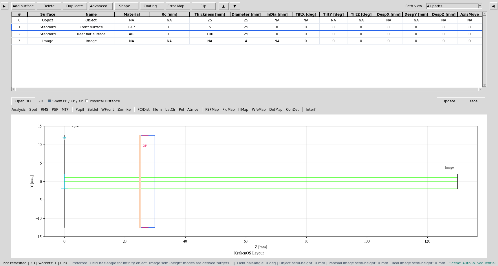
Starting state: Object, BK7 front surface, AIR rear surface, and Image.

Make The Front Surface Variable

1. Right-click the front surface Rc cell.

2. Choose Optimization / Solves -> Select Radius for optimization.

3. Right-click the same Rc cell again and choose Set bounds....

4. Use a positive radius range, for example 20, 100 mm.

The cell should show the Zemax-style V marker. This means the front curvature is now a variable.

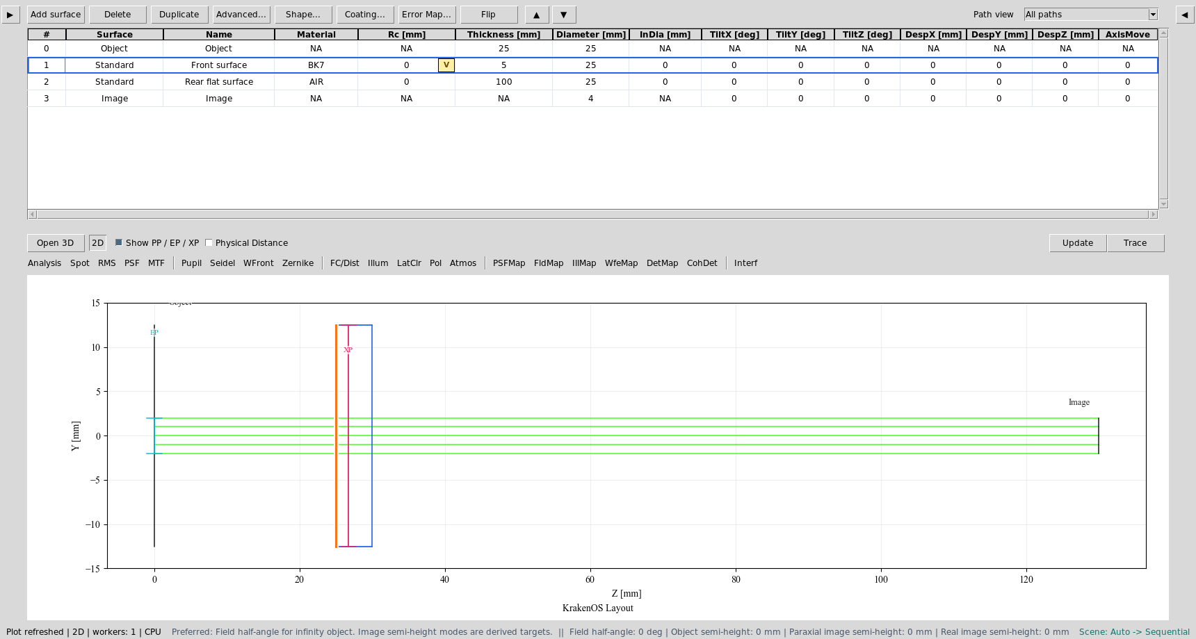
The front Rc cell is selected as an optimization variable and shows the V marker.

Set The EFFL Target

In the Optimization panel:

1. Select the EFFL merit operand.

2. Set Target to 100.

3. Keep Weight at 1 for this simple case.

4. Click Start Optimization.

For BK7 near the visible range, a 100 mm PCX lens with a flat rear surface will usually converge to a front radius around 52 mm. The exact number depends on the active wavelength and glass catalog index.

At this point the table has become a PCX lens prescription, but the image plane may still be wherever the temporary rear-surface thickness placed it.

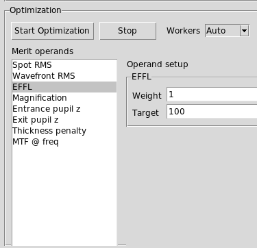
The EFFL operand is selected in the Optimization panel with target 100 mm and weight 1.

Place The Image Plane Correctly

Use one of these two workflows.

Workflow A: solve image distance after EFFL

This is the most beginner-friendly workflow.

1. After EFFL optimization finishes, right-click the rear surface Thickness cell. This is the air distance from the rear lens surface to the Image row.

2. Choose Optimization / Solves -> Paraxial Solve Image Distance.

3. Click Update.

For a 5 mm thick BK7 PCX lens with 100 mm EFFL, the back focal distance is roughly 100 - 5 / n. With BK7 n ~= 1.518, this is about 96.7 mm from the rear surface. The UI should place the Image row near that value for a collimated object-space input.

Workflow B: optimize EFFL and focus together

This is closer to the requested one-button behaviour.

1. Mark the front surface Rc as a variable.

2. Mark the rear surface Thickness as a variable. This controls the image distance.

3. Select the EFFL operand and set target 100.

4. Also select Spot RMS with target 0.

5. Click Start Optimization.

This gives the optimizer two freedoms: bend the front surface to satisfy EFFL, and move the image plane to minimize focus error. Use sensible bounds on both variables so the optimizer cannot choose nonphysical values.

What The User Should See

After the solve:

• The front surface Rc is no longer zero.

• The rear surface remains flat, so the component is plano-convex.

• The material sequence remains BK7 then AIR.

• The 2D plot shows rays converging toward the Image plane.

• The paraxial report should show EFFL near 100 mm.

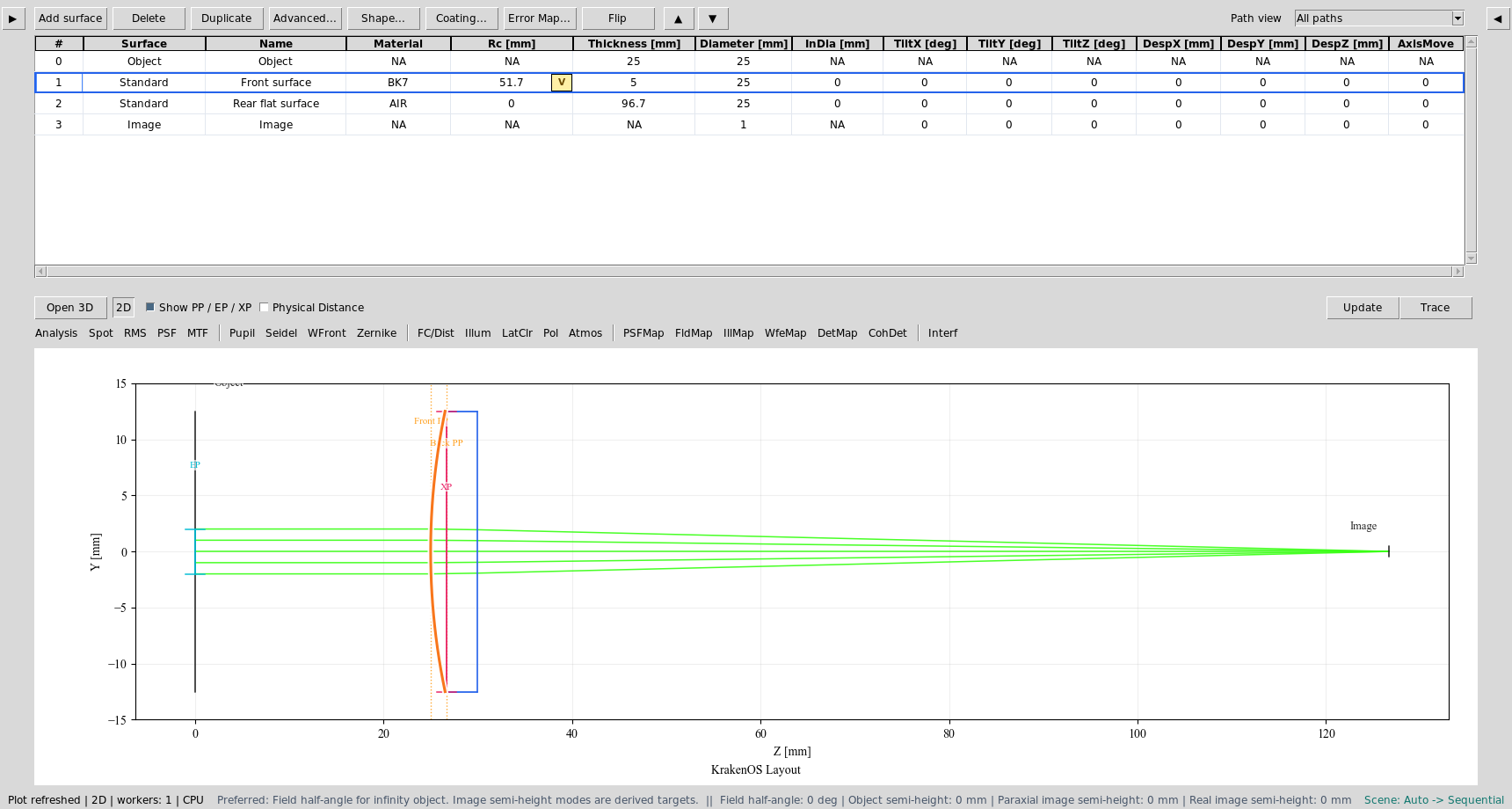
Example solved prescription: front radius about 51.7 mm and rear air-space thickness about 96.7 mm.

Common Mistakes

I selected the front surface as an operand.

In this UI, surfaces are not operands. Surface values are variables; optical results such as EFFL or Spot RMS are operands.

The lens has 100 mm EFFL but the Image row did not move.

This is expected if only front Rc was variable. Run the paraxial image-distance solve or include rear-surface Thickness as a second optimization variable.

The optimizer made a negative or extreme radius.

Add realistic bounds to the Rc variable. For a 100 mm BK7 PCX lens, 20, 100 mm is a reasonable beginner range.

The glass plate did not become a lens.

Confirm the front surface material is BK7 and the rear surface material is AIR. If both are AIR, there is no refractive lens power.