Case Study 5: Mach-Zehnder Two-Output Interferometer

Goal

This case study demonstrates a cascaded beam-splitter workflow:

• load a Mach-Zehnder layout with two physical output ports;

• read the five path labels in the 2D plot;

• isolate each output port with Path view;

• run detector, coherent detector, interferogram, and branch-field analyses;

• verify that the return output port is also available for analysis.

The screenshots in this tutorial are generated from the live Tk UI with:

python -m KrakenOS.UI.capture_mach_zehnder_case_study_screenshots

Load The Mach-Zehnder Layout

1. Start the UI with python -m KrakenOS.UI.layout_editor.

2. Choose Layouts -> Beam Splitters / Folds -> Mach-Zehnder Interferometer (Interferogram).

3. Keep Trace mode = Non-Sequential Preview.

4. Keep NS probabilistic coating split off.

This layout uses two deterministic 50/50 beam splitters. BS1 splits the input source into the upper transmitted arm and lower reflected arm. BS2 recombines those two arms and sends light to two detector ports.

The Object row is a scene/reference datum. Rays launch from the physical Source panel, so source position, radius, direction, power, and ray count control this example.

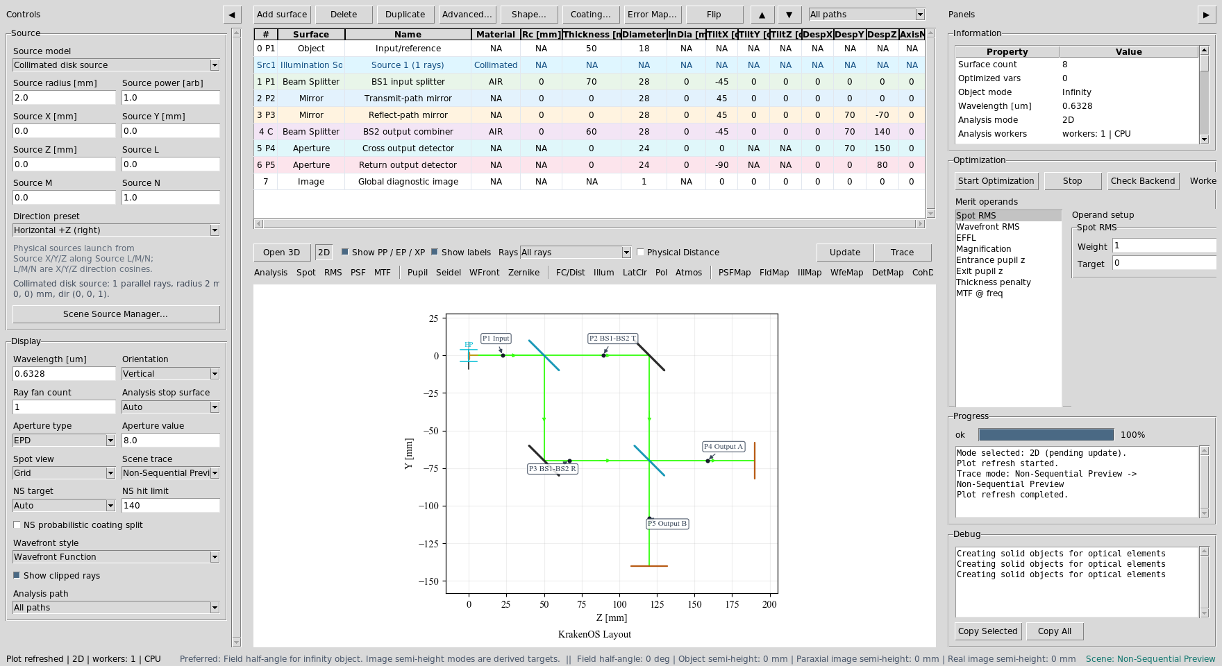
The preset contains a physical source, BS1, two fold mirrors, BS2, a cross-output detector, and a return-output detector.

Read The Path Labels

Click Update. With the default chief-ray source, the 2D plot is intended to read like a schematic. The black-dot labels identify the physical path segments where the user can reason about adding optical components.

Plot label	Meaning
P1 Input	Source to BS1.
P2 BS1-BS2 T	BS1 transmitted arm to BS2.
P3 BS1-BS2 R	BS1 reflected arm to BS2.
P4 Output A	Cross output from BS2 to detector A.
P5 Output B	Return output from BS2 to detector B.

Path labels follow physical legs, not only branch codes. This is the convention used by the table Path view dropdown.

Use Path View For Each Output

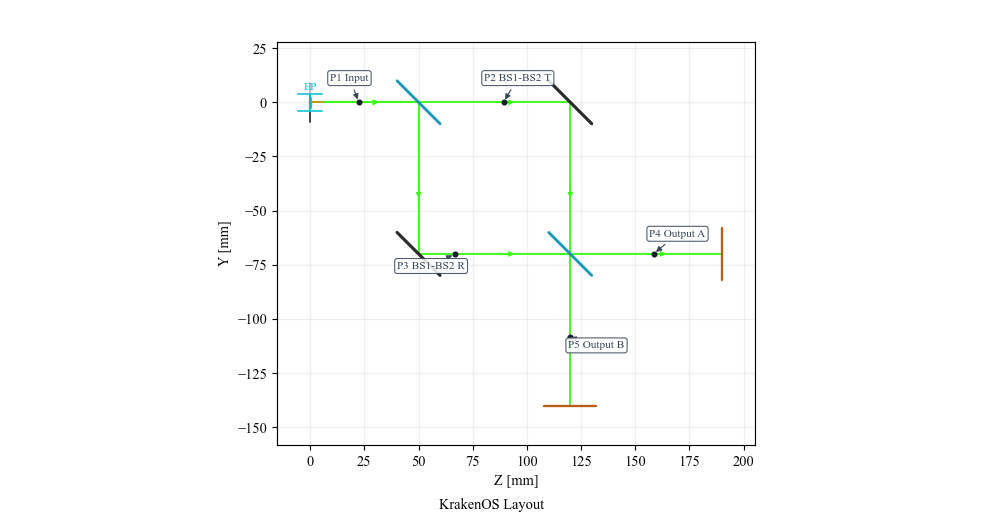
After Update, open the table toolbar Path view dropdown and select:

Path 4: BS2 to cross output detector

This filters the table and plot to the common path plus output detector A. This is the path where branch codes RT and TR recombine.

Path view isolates output A without renumbering the underlying KrakenOS surface rows.

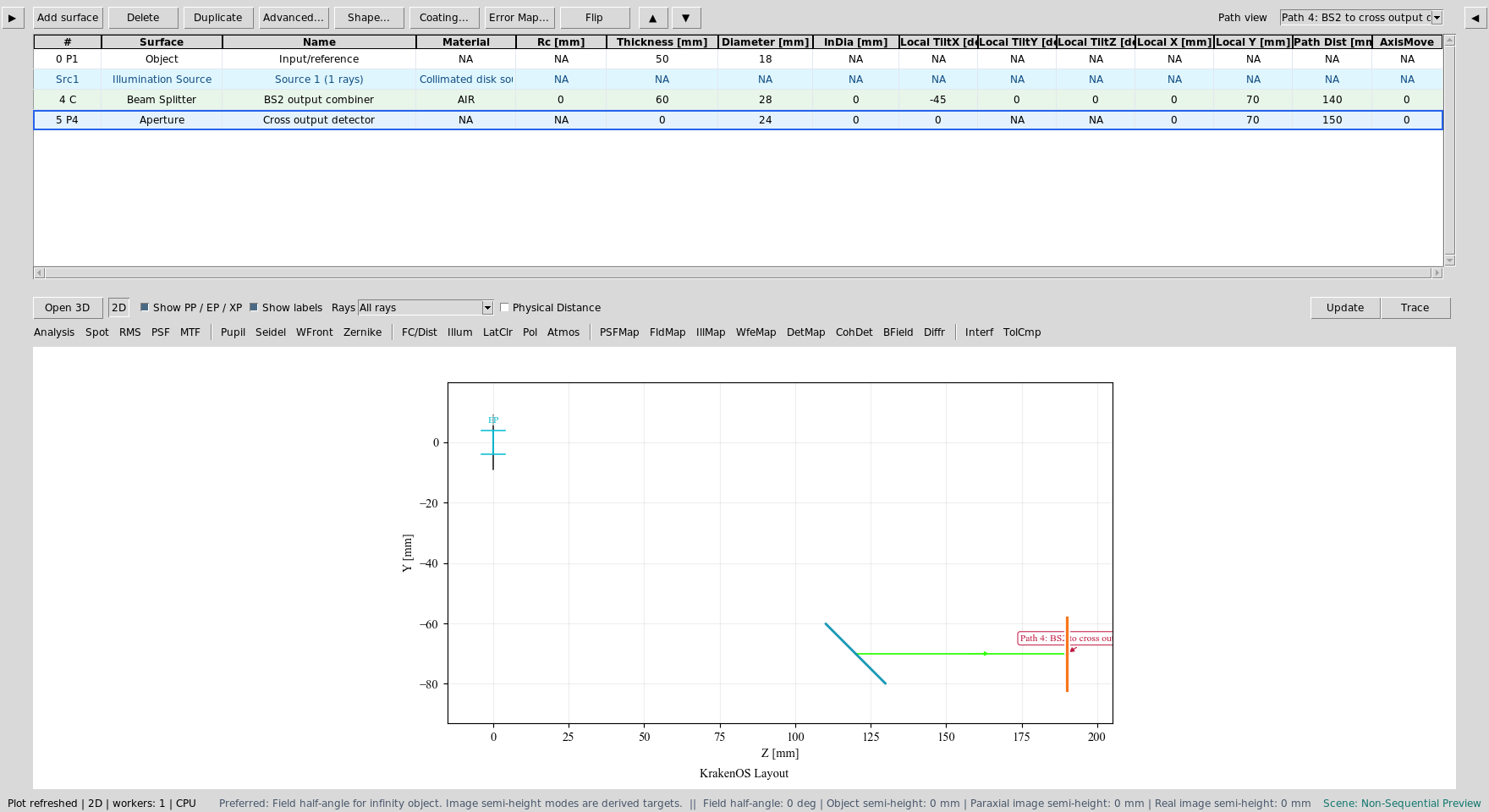
Now select:

Path 5: BS2 to return output detector

This filters the table and plot to the common path plus output detector B. This is the path where branch codes RR and TT recombine.

Output B is a separate detector path, so it can be inspected and optimized independently from output A.

Run Detector Analyses

For analysis screenshots, use a denser source bundle:

Ray fan count = 121
Source radius [mm] = 4.0
Detector bins = 128
Coherent sum = Mutual coherent
Path view = All paths
Analysis path = Output: Detector output port

Click DetMap and Update. This maps detector power at output A.

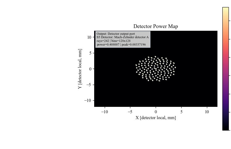
DetMap verifies that both recombining branches reach detector A.

Click CohDet and Update. This uses the same detector hits but sums the complex Jones field by coherence group instead of only summing power.

CohDet reports the detector, branch codes, ray count, and polarization model used for the coherent sum.

Show The Interferogram

Click Interf and Update.

The Mach-Zehnder preset stores interferogram settings on BS2. The interferogram analysis uses the selected detector-output branch family and the saved detector settings to display a detector-bin coherent interferogram.

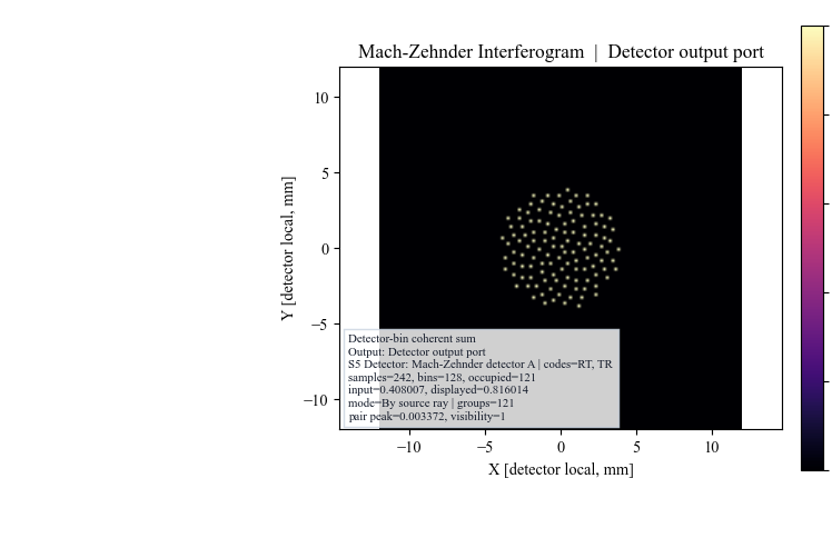
The plotted interferogram is sampled from traced detector hits. Increase source samples and detector bins when a smoother display is needed.

Run Branch Field

Set BField z [mm] = 0. Click BField and Update.

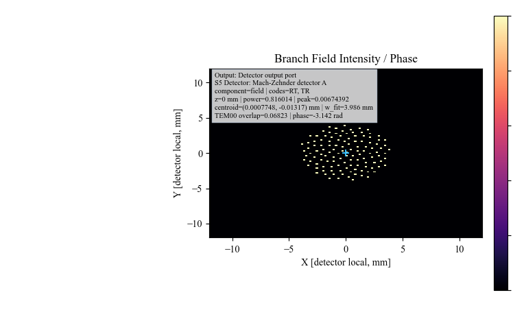
BField promotes the coherent detector samples into a branch-field grid and reports intensity, phase, centroid, and mode diagnostics.

Check The Return Output

Change only the analysis filter:

Analysis path = Output: Source return port

Click CohDet and Update. Output B uses the complementary branch pair, so its branch codes differ from output A.

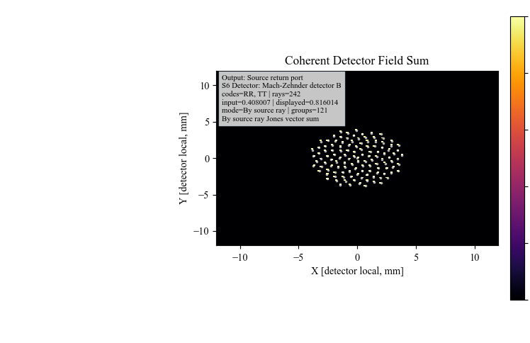
The return-output detector is a first-class analysis target, not a hidden byproduct of the cross-output port.

What This Proves

This case study exercises the non-sequential beam-splitter workflow beyond the single-output Michelson example:

• cascaded beam splitters;

• source/object separation;

• five physical path labels in the 2D plot;

• table filtering by each physical output path;

• two detector output ports;

• detector power analysis;

• coherent field recombination;

• interferogram generation;

• branch-field intensity/phase analysis.

Common Mistakes

I expected Path view to show only one branch code.

Path view follows physical legs. A detector-output leg can contain multiple recombining branch codes.

I selected All paths for coherent analysis and got the wrong output.

For a two-output interferometer, use Analysis path to choose the output port before running coherent detector, interferogram, or branch-field views.

The detector pattern is sparse.

Increase Ray fan count and Detector bins for analysis. Keep Ray fan count = 1 when you want the clean schematic view.

The Object row moved but the source did not.

This preset launches from the Source panel. Move the source controls when you want to move illumination.