Gaussian Beam Propagation

KrakenOS now exposes a lightweight Gaussian beam propagation path on top of the same paraxial matrices used by system.ParaxMatrices() and Actions -> Paraxial Matrix Report. It is intended for first-order laser layout work: waist size, beam radius, divergence, Rayleigh range, wavefront radius, Gouy phase, and CSV export at every paraxial step.

The implementation uses the conventional complex beam parameter:

\[q_{out} = \frac{A q_{in} + B}{C q_{in} + D}\]

where A, B, C, and D are the step matrix values in the (height, angle) convention. KrakenOS refraction matrices include refractive index transitions, so a flat air-to-glass interface scales the Rayleigh range correctly.

Input conventions

All distances are in millimeters. Wavelength is in micrometers, matching the rest of KrakenOS.

Source X/Y/Z and Source L/M/N: The Gaussian source can be launched from a physical origin and chief-ray direction. Source L/M/N are normalized direction cosines. The traced representative rays follow that direction, so the source can be separated from the Object reference row for beam-splitter geometry. The amber q-envelope overlay is intentionally limited to centered +Z paraxial layouts; for tilted or folded Gaussian systems, use the traced rays and the Gaussian Beam Report until the future non-sequential astigmatic q model is implemented.
GB input mode: Waist + offset is the direct q-parameter workflow. Diameter + divergence is the laser-datasheet workflow: enter the beam diameter at the source/reference plane and the full far-field divergence, then KrakenOS back-calculates the equivalent waist radius and waist location.
Cone half-angle [deg]: This is not the Gaussian divergence field. It belongs to geometric random source models such as Random point cone and random area sources. Edit it in Scene Source Manager.... It is a half-angle in degrees, so the full geometric cone angle is twice the entered value.
waist_radius_mm: The 1/e^2 Gaussian field radius at the input waist.
waist_offset_mm: The signed real part of the input q parameter. A value of 0 means the waist is located exactly at the first paraxial input plane. A positive value means the input plane is downstream of the waist. A negative value means the waist is downstream of the input plane.
m2: Beam quality factor. m2=1 is diffraction-limited. Larger values increase the effective wavelength used by the q-parameter report.

Datasheet diameter/divergence flow

Laser manufacturers often specify a beam diameter at the laser output and a full-angle divergence. Use this flow for beam expanders and collimators:

Choose Source model -> Gaussian beam.
Set GB input mode -> Diameter + divergence.
Enter GB diameter [mm] as the 1/e^2 beam diameter at the source plane.
Enter GB full div [mrad] as the full far-field divergence angle.
Choose GB waist side. Waist before source is the normal diverging laser-output case. Waist after source represents a converging beam.
Set GB M2 if the laser is not diffraction-limited.
Click Update. The UI computes the equivalent w0 and waist offset, traces representative rays, and draws the amber 1/e^2 q-envelope.

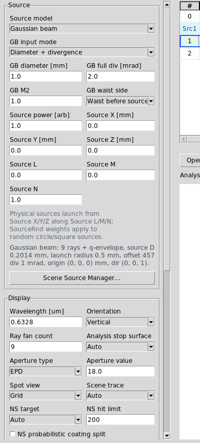
Source panel configured for Gaussian beam diameter and divergence input — In `Gaussian beam` mode, the Source panel shows the laser-datasheet inputs and hides irrelevant pupil/field controls.

The calculation uses:

\[\theta = \frac{\Theta_{full}}{2}\]

\[w_0 = \frac{M^2 \lambda}{\pi n \theta}\]

\[z_R = \frac{\pi n w_0^2}{M^2 \lambda}\]

\[z = z_R \sqrt{\left(\frac{w}{w_0}\right)^2 - 1}\]

where w is half the specified beam diameter at the source plane. If w < w0, the diameter/divergence pair is physically inconsistent and the UI reports an invalid Gaussian source input.

Report columns

Re(q) and Im(q): Complex beam parameter after the paraxial step. Im(q) is the local Rayleigh range in the current medium.
w and 2w: Gaussian beam radius and diameter at the current step.
Rwf: Wavefront radius. inf means a flat wavefront at the waist.
w0: Waist radius implied by the current q state in the current medium.
Waist offset: Distance from the current step plane to the waist. Positive values mean the waist is still downstream of the current step.
Div: Far-field half-angle divergence in milliradians.
Gouy: Gouy phase in radians for the current q state.

Astigmatic and elliptical beams

KrakenOS also exposes a two-axis helper for laser sources whose tangential and sagittal beam diameters, divergences, or M2 values are different. This is useful for diode lasers and beam-shaping lenses where the source is elliptical.

The current UI and ParaxMatrices() path use one centered ABCD sequence, so the two axes differ because the input beam data differ. Branch-carried Gaussian q propagation has a Phase 8B validation baseline for oblique mirrors and first-order oblique refractive powers, but it is not yet a full thick tilted plate or non-sequential wave-optics model. When future non-sequential or tilted surface matrices expose separate tangential/sagittal ABCD chains, the same per-axis propagation routine can consume them.

For splitter and folded-laser future work, see Beam Splitters. Deterministic beam-splitter ray branches now carry power and phase metadata. Ray Inspector and Trace Path Inspector CSV exports now also carry branch-local Gaussian frame columns at every traced hit:

GB K: The local propagation axis for the outgoing branch after that hit.
GB T: The local tangential axis. When a surface normal is available this is the projection of the normal into the plane perpendicular to GB K.
GB S: The local sagittal axis, perpendicular to the local plane of incidence. The frame is right-handed, so GB T x GB S = GB K.
Inc [deg]: The unsigned incidence angle between incoming ray direction and surface normal. It is blank when no reliable surface normal exists.

These columns are the first non-sequential Gaussian contract. KrakenOS also provides KrakenOS.propagate_branch_gaussian_q(record, beam, surfaces=rows) for traced branch records. It propagates independent tangential/sagittal q states, branch distance, optical path, beam radii, wavefront radii, and cumulative centered aperture/obscuration clipping.

The UI exposes the same contract through Actions -> Branch Gaussian Q Report. The report lists one row per branch hit with the q-update note, tangential/sagittal surface powers, q states, beam radii, clipping, and stability flags. Use its CSV export when auditing oblique powered refraction, flat tilted-plate q-only diagnostics, or TIR-deferred cases.

astigmatic_beam = Kos.astigmatic_gaussian_beam_from_diameter_divergence(
    wavelength_um=0.6328,
    tangential_beam_diameter_mm=1.2,
    tangential_full_divergence_mrad=0.9,
    sagittal_beam_diameter_mm=0.8,
    sagittal_full_divergence_mrad=1.4,
    tangential_m2=1.1,
    sagittal_m2=1.3,
    waist_after_input=False,
)
astigmatic_trace = Kos.propagate_astigmatic_gaussian_beam(
    paraxial_trace,
    astigmatic_beam,
)
print(astigmatic_trace.final_tangential.beam_radius_mm)
print(astigmatic_trace.final_sagittal.beam_radius_mm)

Validate the branch-frame contract with:

python -m KrakenOS.UI.validate_gaussian_branch_frames

Validate branch-carried q and detector-side Gaussian recombination with:

python -m KrakenOS.UI.validate_gaussian_branch_q
python -m KrakenOS.UI.validate_gaussian_detector_recombination

For active Source-panel Gaussian interferometer layouts, the Interf analysis uses the branch-carried q envelope and cumulative clipping when detector-bin coherent promotion is reliable. The displayed annotation reads Gaussian-q detector-bin coherent sum. This is a detector-bin geometric field model.

Phase 8 branch-field propagation

Phase 8 starts the higher-order field-propagation layer with a small reusable contract in KrakenOS.BranchField. The first helper is scalar and grid-based: it is designed to sit between traced branch/detector data and future UI field plots without adding more analysis logic directly to the editor.

BranchFieldGrid: A complex scalar field sampled on monotonic x_edges_mm and y_edges_mm. The first contract uses the same discrete power convention as CohDet and Diffr: sum(abs(field)**2).
BranchFieldGrid.centroid_mm(): Returns the intensity-weighted sampled field centroid. The UI uses this as the center for the first fitted TEM00 overlap estimate.
make_gaussian_tem00_field(...): Builds a normalized waist-plane TEM00 field on a rectangular grid.
propagate_branch_field(grid, distance_mm): Propagates the scalar field through homogeneous free space using a unitary paraxial/Fresnel transfer function. This conserves the discrete field power to numerical precision.
gaussian_mode_overlap(grid, waist_radius_mm=...): Computes normalized overlap efficiency against a waist-plane TEM00 reference sampled on the same grid.
branch_field_from_detector_data(data, component=...): Converts current coherent-detector data dictionaries into the Phase 8 field contract. This is the bridge from Phase 7 detector-bin fields to future branch-field plots.

Minimal API example:

import numpy as np
import KrakenOS as Kos

x_edges = np.linspace(-4.0, 4.0, 129)
y_edges = np.linspace(-4.0, 4.0, 129)
field = Kos.make_gaussian_tem00_field(
    x_edges_mm=x_edges,
    y_edges_mm=y_edges,
    wavelength_um=0.6328,
    waist_radius_mm=0.55,
    power=1.0,
)
propagated = Kos.propagate_branch_field(field, 250.0)
overlap = Kos.gaussian_mode_overlap(propagated, waist_radius_mm=0.55)
print(propagated.total_power)
print(overlap.efficiency)

Run the example and validators with:

python KrakenOS/Examples/Examp_Branch_Field_Propagation.py
python -m KrakenOS.UI.validate_phase8_field_contract
python -m KrakenOS.UI.validate_phase8_complete

The UI-facing entry point is the BField analysis button beside CohDet and Diffr. It reuses the selected Analysis path and detector-bin count, promotes the coherent detector samples into BranchFieldGrid, then plots:

normalized scalar field intensity,
wrapped phase contours in radians where the field has enough power,
the fitted intensity centroid,
a TEM00 overlap estimate using the second-moment radius as the fitted waist.

The BField z [mm] field in the left analysis controls applies the first Phase 8 paraxial propagation helper before plotting and measuring the field. Use 0 for the detector plane. Positive and negative distances are accepted for forward/backward propagation on the same sampled grid. Actions -> Export Branch Field CSV... writes one row per field bin with complex field, intensity, phase, propagation distance, centroid, fitted waist, and TEM00 overlap metadata.

Headless snapshot example:

python -m KrakenOS.UI.render_layout_snapshot \
  --file KrakenOS/common_optical_layouts/michelson_interferometer_ray_only.py \
  --mode branch_field \
  --output testing/branch_field.png

This first slice is intentionally not a full tilted thick-plate field propagator. Fully oblique astigmatic matrices and richer mode-overlap workflows remain Phase 8 follow-up slices.

Phase 8B oblique astigmatic q baseline

Phase 8B validates the branch-carried Gaussian-q surface-power contract. The current behavior is:

flat mirrors/folds behave as pure branch-local free-space q propagation,
flat oblique refractive plate faces are marked as q-only index steps, not full tilted-plate field propagation,
oblique spherical reflection applies different tangential and sagittal curvature powers,
near-normal spherical refraction applies symmetric first-order power,
oblique spherical refraction applies first-order Coddington tangential and sagittal powers in the branch-local frame,
above-critical synthetic transmit hits are marked as TIR-deferred q diagnostics instead of silently applying a spherical power.

The validator also loads the real Galvo F-Theta Laser Scanner common layout, runs the same headless UI trace used by the ray inspector, and checks that traced oblique refractive hits match the first-order tangential/sagittal surface powers.

Run the diagnostic example and validator with:

python KrakenOS/Examples/Examp_Oblique_Astigmatic_Q.py
python -m KrakenOS.UI.validate_phase8b_complete
python -m KrakenOS.UI.validate_branch_gaussian_q_report
python -m KrakenOS.UI.validate_oblique_astigmatic_q
python -m KrakenOS.UI.validate_phase8_complete

Phase 8B is closed at this Gaussian-q contract scope. This is still a first-order q update at traced surface hits. Flat oblique refractive plates are labeled as q-only index steps; they do not yet replace full wave propagation through thick tilted splitter plates or arbitrary CAD prisms. That work belongs in a later branch-field/physical-optics layer, not another silent q-only patch.

Cavity eigenmode flow

The Gaussian Beam Report includes a Use Cavity Eigenmode button. It solves the self-consistent mode:

\[q = \frac{Aq + B}{Cq + D}\]

for the current ABCD matrix, then fills the report input waist and waist offset with that eigenmode. Use this only when the current ABCD matrix represents one complete cavity round trip at the chosen reference plane. A normal single-pass imaging lens is not a cavity round trip, so the button may correctly report an unstable or invalid eigenmode.

The reported stability parameter is:

\[g = \frac{A + D}{2 \sqrt{AD - BC}}\]

and the mode is stable when |g| < 1 and the solved q has a positive imaginary part.

The same solve is available from Python:

import numpy as np
import KrakenOS as Kos

L = 300.0
R = 1000.0
propagation = np.array([[1.0, L], [0.0, 1.0]])
mirror = np.array([[1.0, 0.0], [-2.0 / R, 1.0]])
round_trip = mirror @ propagation @ mirror @ propagation

mode = Kos.solve_gaussian_cavity_eigenmode(
    round_trip,
    wavelength_um=0.6328,
    m2=1.0,
)
if mode.stable:
    beam = mode.beam
    print(beam.waist_radius_mm, beam.waist_offset_mm)

UI workflow

Load Common Optical Layout -> Gaussian Beam ABCD Example.
In the Source panel, choose Gaussian beam.
Set GB waist [mm], GB waist offset [mm], and GB M2.
Click Update to trace representative Gaussian source rays and draw the amber 1/e^2 q-envelope in the 2-D layout.
Open Actions -> Gaussian Beam Report for the per-surface q table.
For resonator layouts whose ABCD matrix is one complete round trip, click Use Cavity Eigenmode to seed the report from the stable cavity mode.
Use Export CSV when you want to compare the per-step q trace externally.

Low ray-count Gaussian previews use equal-spaced meridional samples inside the current beam radius so the 2-D layout gaps are uniform. The outer preview rays stay conservatively inside the source edge to avoid accidental clipping on tilted finite plates. Increase Ray count above nine when you want the representative rays to fill the 2-D source disk.

Folded laser scanner example

Common Optical Layout -> Galvo F-Theta Laser Scanner demonstrates a typical laser-scanner path:

a Gaussian 650 nm source using diameter/divergence input (1 mm beam diameter and 2 mrad full divergence in the preset);
a negative/positive two-lens beam expander tuned for about 2x expansion, so the beam at the galvo/entrance stop is compatible with the Figure 8 2 mm EPD;
a 45 degree galvo mirror;
a 50 mm F-theta lens transcribed from attachment/F-theta.pdf Figure 8;
a flat scan/focus plane.

The preset uses Folded Preview plus explicit Folded reach = Display compatibility so the 2-D layout reads like the physical bench: beam expander, fold mirror, downward F-theta leg, and scan plane. That detector reach mode is legacy display compatibility; exported ray records still mark the folded terminal provenance. The case is also covered by the branch-frame and branch-q validators, so it is useful for checking folded Gaussian q propagation contracts. It is still not a higher-order diffraction or mode-overlap field solver. The F-theta lens data is also available as Common Optical Layout -> F-Theta Lens 50mm Figure 8. Its original Zemax K9 glass is mapped to bundled CDGM H-K9L.

The galvo mirror row also supports a 2-D scan overlay directly in the prescription table. Edit the mirror TiltX cell and enter comma-separated values, such as 40,45,50, or a range like 40:50:5. These values use the same displayed mirror angle as the table cell; they are not the optical F-theta field angle. Around the 45 degree fold, the optical scan angle is twice the displayed mirror-slant change from the nominal 45 degree fold. Thus 40,45,50 is a conservative -10,0,+10 degree optical scan. The Figure 8 prescription is a 40 degree full-field lens, so its nominal full optical scan is -20,0,+20 degrees, entered as 35,45,55. The middle value becomes the nominal pose stored on the row; the full list draws additional mirror positions and representative focused bundles without duplicating rows in the prescription table. The right-click Galvo scan overlay... dialog edits the same setting.

For a step-by-step UI walkthrough with reproducible snapshots, see Case Study 17: Galvo F-Theta Laser Scanner.

Other pose cells use the same comma/range syntax for mechanical tolerance overlays. For example, entering -0.05,0,0.05 in a lens DespX cell keeps 0 as the nominal prescription value and overlays the decentered ray traces in the 2-D plot without duplicating lens rows.

If the folded scanner spot is not exactly on the scan plane, first validate the standalone F-Theta Lens 50mm Figure 8 layout with object mode Infinity. The integrated scanner also includes a finite Gaussian source and beam expander; its exact plane focus depends on the expander collimating the beam at the galvo/entrance stop.

Python example

The same feature is available directly from Python:

import KrakenOS as Kos

setup = Kos.Setup()

obj = Kos.surf()
obj.Name = "Input plane"
obj.Thickness = 80.0
obj.Diameter = 20.0
obj.Glass = "AIR"

lens = Kos.surf()
lens.Name = "Focusing lens f=100"
lens.Thin_Lens = 100.0
lens.Thickness = 130.0
lens.Diameter = 30.0
lens.Glass = "AIR"

image = Kos.surf()
image.Name = "Readout plane"
image.Thickness = 0.0
image.Diameter = 16.0
image.Glass = "AIR"

system = Kos.system([obj, lens, image], setup)
paraxial_trace = system.ParaxMatrices(0.6328)

beam = Kos.GaussianBeamInput(
    wavelength_um=0.6328,
    waist_radius_mm=0.5,
    waist_offset_mm=0.0,
    m2=1.0,
)

# Alternative manufacturer-style input:
beam = Kos.gaussian_beam_from_diameter_divergence(
    wavelength_um=0.6328,
    beam_diameter_mm=1.0,
    full_divergence_mrad=1.0,
    m2=1.0,
    waist_after_input=False,
)
beam_trace = Kos.propagate_gaussian_beam(paraxial_trace, beam)

for step in beam_trace.steps:
    print(
        step.step_index,
        step.label,
        f"w={step.beam_radius_mm:.6g} mm",
        f"R={step.wavefront_radius_mm:.6g} mm",
        f"waist_offset={step.waist_offset_mm:.6g} mm",
    )

A runnable version of this example is available at KrakenOS/Examples/Examp_Gaussian_Beam_Propagation.py. A second runnable example for astigmatic beams and cavity eigenmodes is available at KrakenOS/Examples/Examp_Gaussian_Laser_Modes.py.

Scope and limitations

This is a q-parameter and detector-bin Gaussian envelope tool, not a full diffraction field propagator. Branch q traces include centered aperture/obscuration clipping, and promoted Gaussian-source interferograms can use detector-bin coherent recombination. Higher-order modes, FFT propagation through arbitrary clipping, and true tilted thick-plate mode-overlap still require future wave-optics work. Tangential/sagittal helpers model independent two-axis source data on the current centered ABCD path; fully oblique astigmatic optics still require future separate axis matrices.

The 2-D layout also traces an exact-count representative 2-D disk bundle so the source appears in the normal ray display. The amber envelope is the physical Gaussian beam size; the traced rays are still a visual/geometric guide rather than a diffraction-field calculation.

Source-mode field relevance

When Gaussian beam or another physical source is selected, object/field and pupil controls do not define the source. The UI therefore hides unused controls such as Object mode, Field type, Pupil pattern, and Pupil factor. The saved values are preserved internally and restored when returning to Pupil / field.

This distinction is intentional for future beam-splitter and illumination workflows: an illumination source is a separate entity from the optical object. For example, a source can illuminate an object through a 45 degree beam splitter from a 90 degree direction. In that case source position, direction, beam diameter, divergence, and power define the launched rays; object mode and pupil-factor ray-height scaling are not the ray-generation controls.