Case Study 9: Tolerance Monte Carlo And Compensators

Goal

This case study shows the tolerance workflow that follows an optimized nominal design:

• load a layout with native KrakenOS variables already marked;

• sample manufacturing perturbations with a deterministic Monte Carlo run;

• keep one variable as a compensator and one variable as tolerance-only;

• couple both variables to one physical manufacturing source;

• inspect worst-sample, stack-up, and compensator reports;

• verify the same result visually with the TolCmp analysis button.

The screenshots in this tutorial are generated from the live Tk UI with:

python -m KrakenOS.UI.capture_tolerance_monte_carlo_case_study_screenshots

Load The Native-Variable Layout

1. Start the UI with python -m KrakenOS.UI.layout_editor.

2. Choose Layouts -> Advanced Surfaces / Materials -> Native Variable Breadth Example.

3. Keep Object Mode = Infinity.

4. Keep Field Type = Angle, Field Value = 3.0, and Field Count = 3.

5. Keep the Spot RMS merit operand selected.

The important row is S1 Conic / tilt variable surface. It has two marked native variables:

k bounds     = -1.5, 0.5
Tilt X bounds = -3 deg, 3 deg

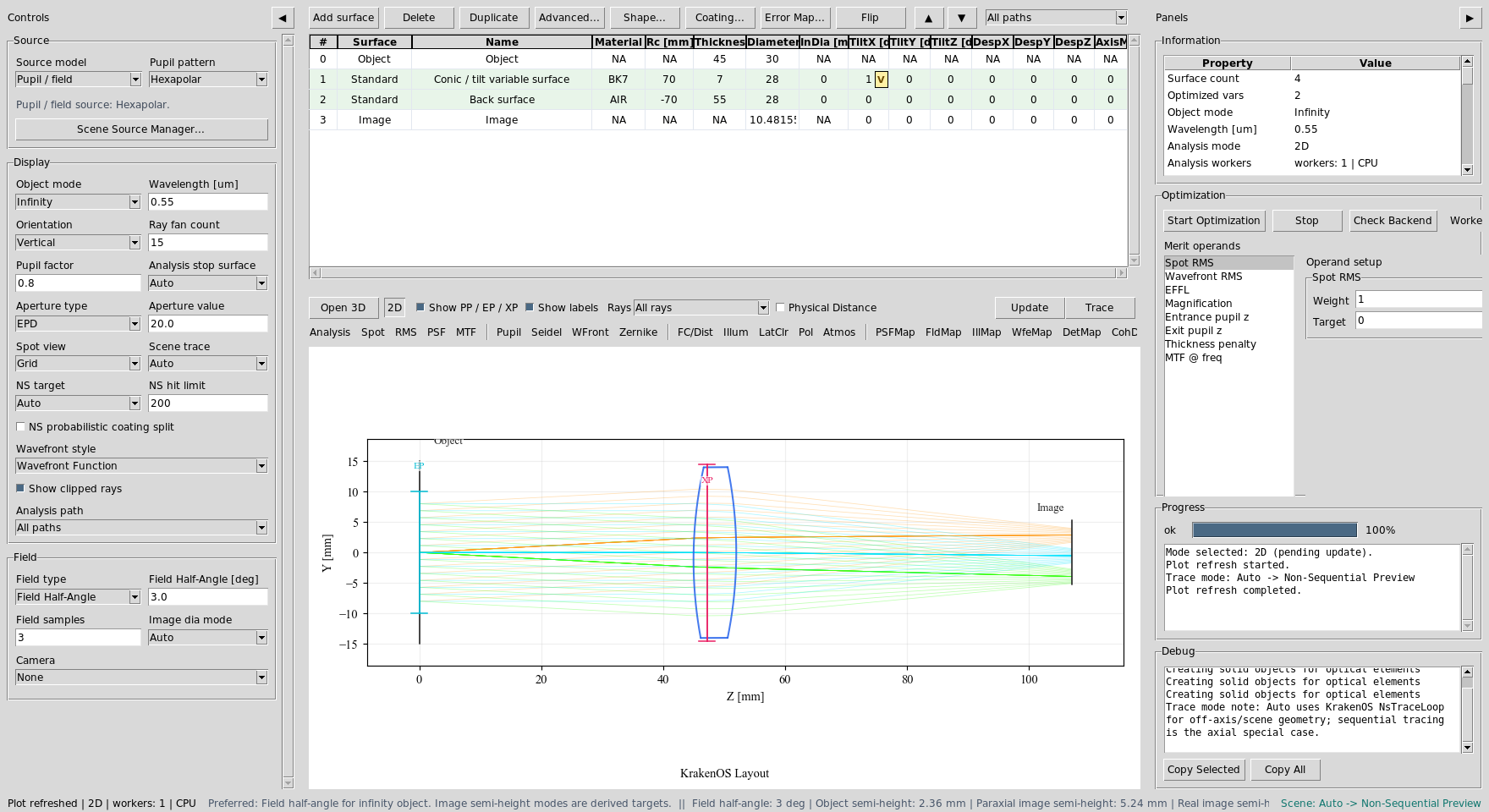
The nominal prescription is small on purpose. The case study focuses on the tolerance workflow, not lens complexity.

Choose Tolerance Roles

Right-click the marked S1 k cell and keep it as a tolerance compensator. Right-click the marked S1 Tilt X cell and choose:

Optimization / Solves -> Do not use TiltX as tolerance compensator

This means both variables are sampled as manufacturing errors, but only k may be moved during compensator sweeps. That is the usual workflow when one parameter can be adjusted during assembly and another is a fixed build error.

Now assign both variables to one manufacturing source:

1. Right-click S1 k and choose Optimization / Solves -> Set tolerance coupling group....

2. Enter shared_mount.

3. Right-click S1 Tilt X and choose the same command.

4. Enter -shared_mount.

The minus sign means Tilt X uses the opposite random quantile of the same sampled manufacturing degree of freedom. This avoids treating one machined mount error as two independent random errors.

Attach manufacturing metadata with:

machined mount | MNT-001 | cell, vendor-a | shared cell machining

Save this as a template named Shared machined mount and apply it to both variables. Reports and CSV exports carry this metadata so an optical tolerance row can be traced back to a real process, drawing, vendor spec, or mount.

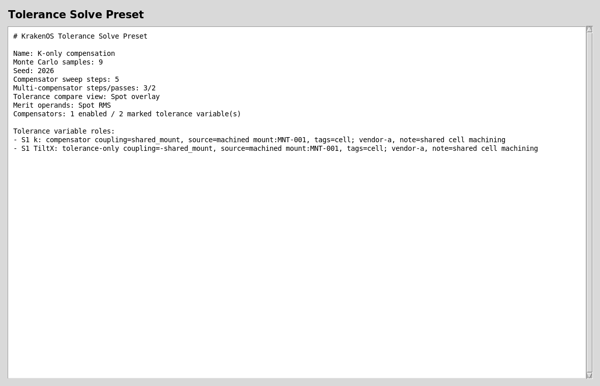
The preset captures sample count, seed, selected operands, compensator eligibility, coupling groups, and manufacturing metadata.

Run Monte Carlo

Choose Actions -> Tolerance Monte Carlo Report.... For this tutorial use:

Monte Carlo sample count = 9
Random seed = 2026

The report samples each marked variable inside its bounds, evaluates the selected merit operand, and leaves the nominal table unchanged.

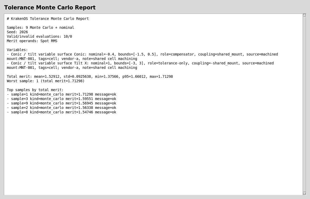
The variable list shows which entries are compensators, which are tolerance-only, which coupling group they belong to, and which manufacturing source generated the tolerance.

Compare The Worst Sample

Choose Actions -> Tolerance Worst-Sample Comparison.... This compares the nominal system with the worst valid perturbed sample from the last Monte Carlo run.

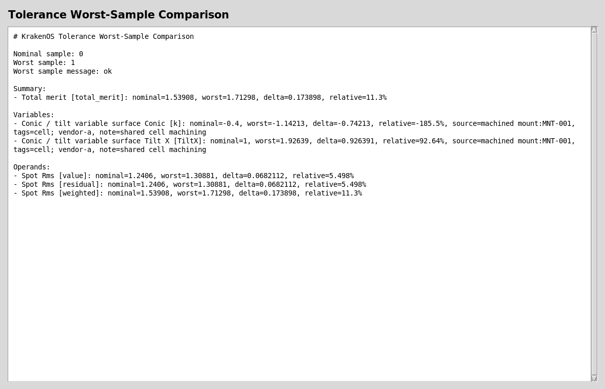
Use this report when you need concrete variable deltas and operand deltas, not only statistical summary values.

Plot The Worst-Sample Spot Overlay

Click TolCmp and set:

Tolerance compare view = Spot overlay

Then click Update.

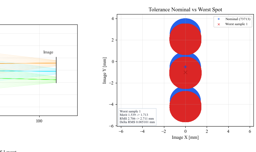
Spot overlay rebuilds temporary nominal and worst-sample systems and overlays their image-plane spot clouds. It does not change the editable table.

Read The Stack-Up Bars

Set:

Tolerance compare view = Stack-up bars

Then click Update.

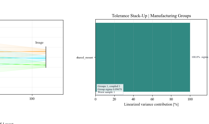
Coupled variables are shown as one manufacturing group. This is the view to use when discussing which physical tolerance source dominates the merit variance.

Run Compensator Sweeps

Choose Actions -> Tolerance Compensator Sweep... and use 5 steps. The UI holds the system at the worst Monte Carlo sample and sweeps each eligible compensator through its bounds.

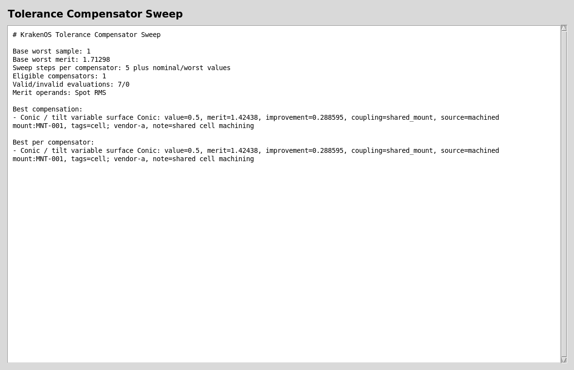
Only k is swept because Tilt X was explicitly marked tolerance-only. The report is diagnostic and does not mutate the nominal prescription.

Choose Actions -> Tolerance Multi-Compensator Solve... to run the same idea as a bounded coordinate solve.

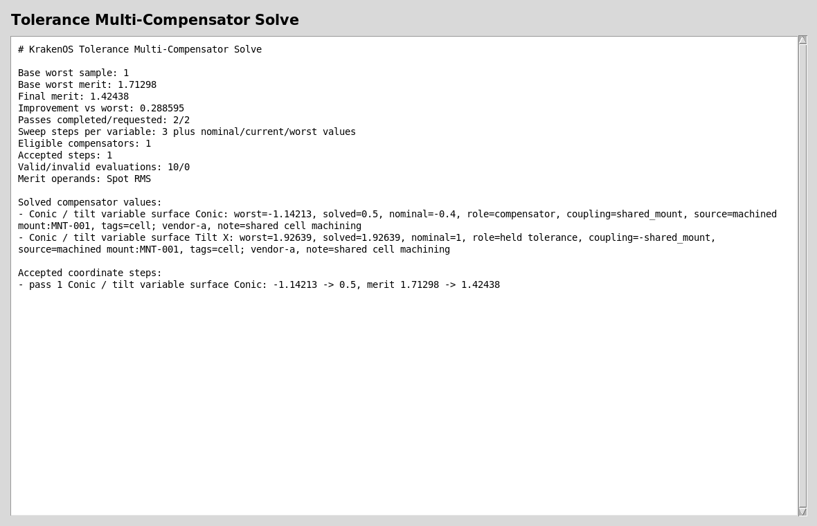
Tolerance-only variables stay fixed at their worst-sample values. Eligible compensators can move only when the move improves the merit.

Check MTF Impact

Set:

Tolerance compare view = MTF overlay

Then click Update.

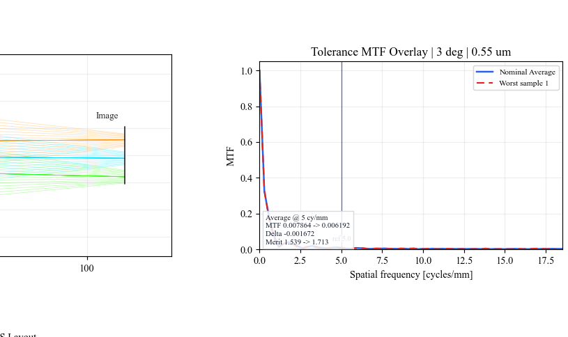
MTF overlay is a quick visual check for whether the worst sample changes contrast at the selected spatial frequency.

Run The Python Example

The same workflow is scriptable:

python KrakenOS/Examples/Examp_Tolerance_Compensator_Sweep.py

The example prints the preset, Monte Carlo, stack-up, compensator sweep, and multi-compensator reports, plus CSV schema summaries for external review.

What This Proves

This case study exercises the Phase 7E tolerance/manufacturing workflow:

• native KrakenOS variable discovery from row advanced["Var"] metadata;

• deterministic Monte Carlo sampling with fixed seed;

• explicit compensator versus tolerance-only roles;

• coupled manufacturing degrees of freedom;

• reusable manufacturing metadata templates;

• worst-sample comparison reports;

• covariance-aware stack-up dashboard;

• single- and multi-compensator diagnostic solves;

• TolCmp spot, stack-up, and MTF overlays.

Common Mistakes

I expected the table values to change after Monte Carlo.

Tolerance runs rebuild temporary systems. The nominal editable table stays unchanged unless you manually accept a design change.

Every variable was swept as a compensator.

By default, marked tolerance variables are eligible compensators. Right-click a marked variable cell and disable compensator use when the variable is a fixed manufacturing error.

The stack-up shows one bar for two variables.

That is correct when both variables share the same coupling group. It means the UI is ranking the physical manufacturing source, not double-counting each row as an independent random error.

The reports mention source=machined mount:MNT-001.

That is manufacturing metadata. It does not change the ray trace, but it makes the tolerance report auditable against a real mount, spacer, vendor process, or drawing.