Case Study 18: One Lens, Many Analyses
Goal
This case study ports the analysis-breadth workflow from Optiland
Tutorial_4b_PSF_&_MTF_Calculation.ipynb and
Tutorial_4c_Zernike_Decomposition.ipynb into one KrakenOS UI sequence. A
single stable infinity-object Double Gauss prescription is used for Spot, PSF, MTF,
Wavefront, and Zernike analysis so the user can learn the analysis panels
without changing the optical design between steps.
The screenshots in this tutorial are generated from the live Tk UI with:
python -m KrakenOS.UI.capture_double_gauss_analysis_case_study_screenshots
The physics validator is:
python -m KrakenOS.UI.validate_double_gauss_analysis_case_study
There is also a scriptable example:
python -m KrakenOS.Examples.Examp_Double_Gauss_Analysis_Suite
Load The Analysis Layout
Start the UI with
python -m KrakenOS.UI.layout_editor.In the top menu, choose
Layouts -> Analysis / Diagnostics -> Double Gauss PSF MTF Wavefront Zernike Case Study.Confirm the controls:
Object Mode = Infinity;Aperture = EPD;EPD = 4 mm;Field Type = Angle;Field Value = 0 deg;Wavelength = 0.55 um;Wavefront Style = Wavefront Function.
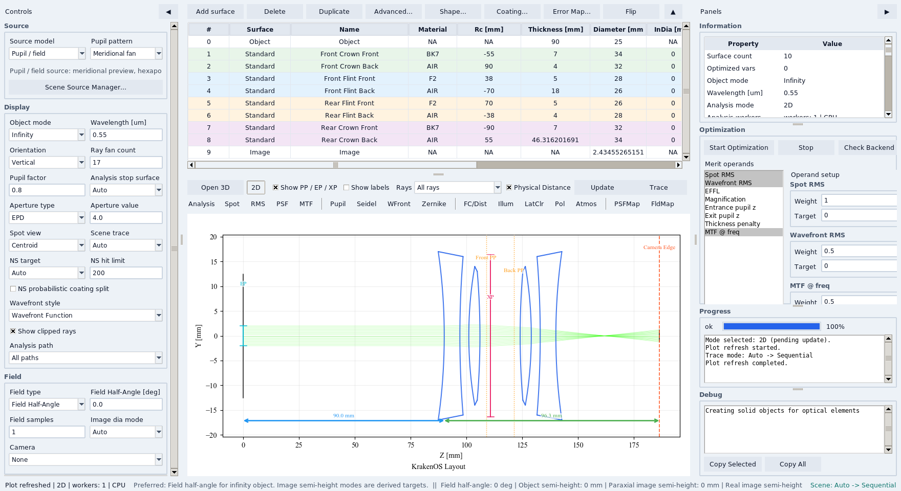
The same infinity-object Double Gauss layout drives all analysis panels.
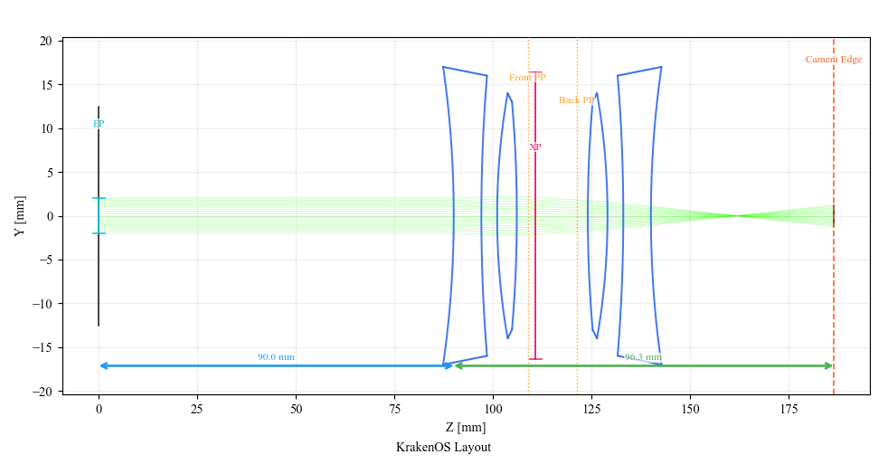
The prescription is conventional and stable, so the tutorial can focus on interpreting the analysis outputs.
Spot: Check Geometric Focus
Click Spot and Update. Use Centroid spot mode for the simplest
first read: the plot is centered on the geometric centroid, making the blur
shape easier to inspect.
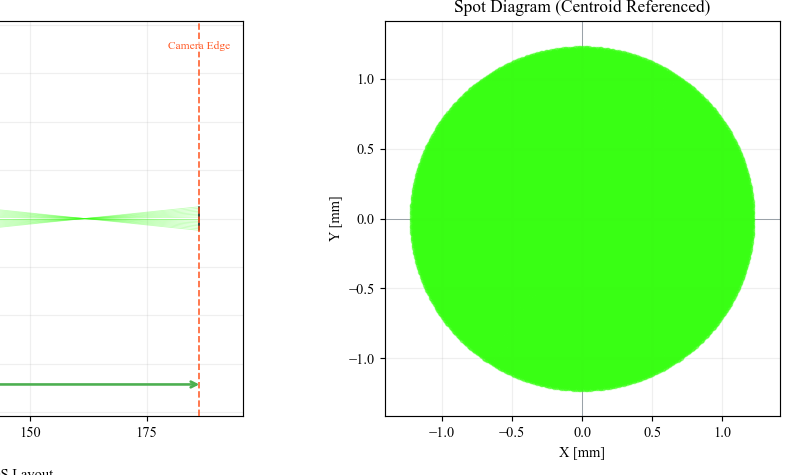
Spot is the fastest sanity check: rays should land in a compact finite cloud at the image plane.
PSF: Convert Samples Into Image Intensity
Click PSF and Update. The current KrakenOS panel is a geometric PSF:
it bins traced image-plane ray intercepts into normalized intensity. This is
not a diffraction PSF, but it is useful for finding blur shape and alignment
errors.
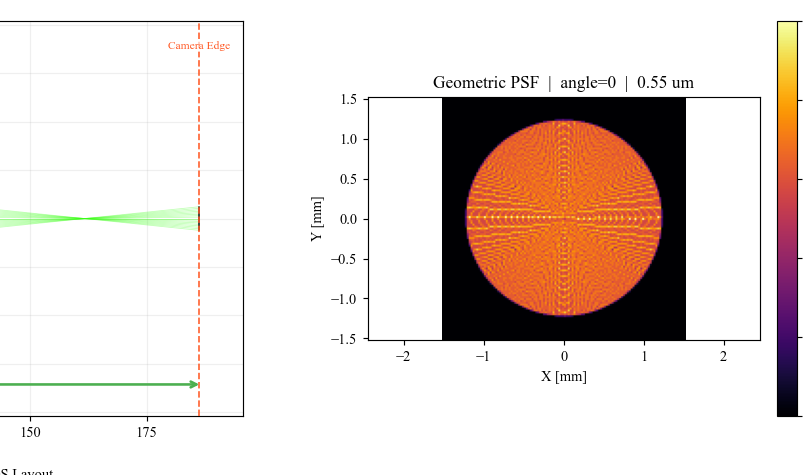
The PSF panel makes the spot distribution easier to compare with detector sampling or image-processing expectations.
MTF: Read Contrast Versus Spatial Frequency
Click MTF and Update. In the Optimization panel, MTF @ freq is
preset to 20 cycles/mm with Alg = PSF FFT. The plot shows tangential
and sagittal curves computed from the same geometric image-plane samples.
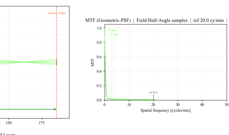
MTF converts the blur cloud into a contrast metric that can be used in a merit function or a presentation checklist.
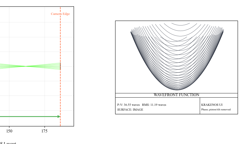
Wavefront: Inspect Pupil Phase
Click Wavefront and Update. Keep Wavefront Style set to
Wavefront Function. This removes piston and best-fit tilt so the plot
emphasizes optical aberration instead of image-plane pointing.
Use File -> Export Wavefront CSV... after this panel has been rendered
if the pupil samples are needed outside the UI.
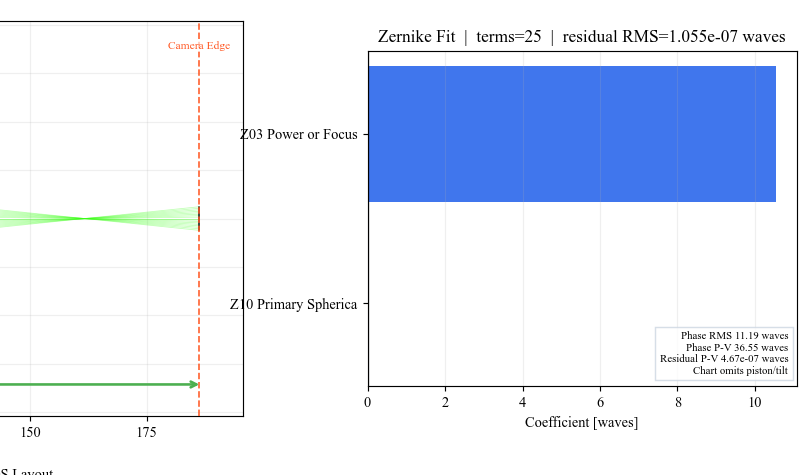
Zernike: Decompose The Wavefront
Click Zernike and Update. The Zernike panel fits the sampled
wavefront and stores both coefficient rows and residual samples for export.
Use File -> Export Zernike CSV... after this panel has been rendered to
capture coefficient values and residual statistics.
What This Proves
This case study is intended for quick review sessions. It proves that one menu-backed sequential lens can drive the main KrakenOS analysis panels, stores exportable wavefront/Zernike data, and gives the user a repeatable workflow before moving to harder non-sequential or coherent examples.