Editable Table Workflow

The editable table is the working prescription for sequential layouts and the surface/object list for non-sequential scene workflows. A single row is a KrakenOS surface. A component is one or more adjacent rows grouped as an Element so that the UI can move, flip, copy, paste, ungroup, and path-tag the optical component as one unit.

Physical illumination sources are already first-class scene objects through the Source panel and SETTINGS["scene_sources"]. Use Actions -> Scene Source Manager... or the Source-panel Scene Source Manager... button to add, edit, delete, duplicate, or reorder explicit physical emitters. When the selected source is a physical emitter, the table shows an Illumination Source scene row beside Object and Image. Double-click that source row to open the manager. Right-click it for direct source-row actions: edit in the manager, duplicate, delete when more than one explicit source exists, or move the source up/down relative to adjacent source rows. The row is not a KrakenOS surface: it has no table-row index, no trace-surface index, and is skipped when the surface prescription is read back for tracing. This preserves KrakenOS surface indices used by ray tracing, path assignment, detectors, and analysis. The source-aware SceneRowMapping bridge records this source-visible row order while the prescription rows remain ordinary KrakenOS surfaces. Layouts may request scene_row_order="before_object" when the source is the intuitive first entity in the workflow, for example a right-angle beam-splitter illumination scene where Source 1 illuminates an object through folded optics.

For a single source, the Source panel remains the quick fallback. For multiple sources, the manager writes explicit scene_sources records. Inspect the exact scene/table/trace mapping in Actions -> Non-Sequential Scene Graph; the graph shows the scene row number, current table row, trace surface, and source ID side by side.

Use Direction preset in the Source panel or Scene Source Manager to orient physical emitters without manually entering direction cosines. Horizontal +Z (right) is the normal left-to-right source direction in the YZ layout; the equivalent manual entry is Source L=0, Source M=0, Source N=1. In Scene Source Manager, Aim Direction At Row points the selected source origin at the center of a chosen Object, surface, Image, or file-backed CAD/STL row. It updates only the source direction cosines, so the source remains a scene emitter and the optical prescription rows are not reordered or modified. When a CAD/STL row has assigned optical face roles, the target dropdown also lists those face anchors, for example 1/F001. Choosing one uses the transformed face centroid instead of the whole mesh center. From the CAD/STL face assignment dialog, Use Face As Source Target saves the selected face roles and opens Scene Source Manager with that face preselected. From the 3D Inspector, Source Target starts a pick mode: click a surface or CAD solid and the manager opens on that row; if the click lands near an assigned CAD/STL optical face, that face anchor is preselected. Place Origin At Standoff uses the current Source L/M/N direction and the chosen target row to set Source X/Y/Z a positive distance upstream of that target. Set a direction preset first when you want a predictable placement such as Horizontal +Z or Vertical -Y.

After tracing, use Actions -> Source Illumination Report to inspect how each physical source illuminates the selected Object, aperture, detector, or Image surface. The report uses traced 3D ray hits and does not add pseudo-surfaces to the prescription. If rays miss the selected target, the report lists missed power plus the dominant terminal/loss surface so you can tell whether the source is being clipped by Object/reference geometry, a stop, a splitter branch, or the detector aperture. Select a source row in the report to read the full loss, power, centroid, RMS, and span details without widening the table columns.

The Illum analysis uses the same source-hit records. In Auto target mode it prefers the final Detector/Image plane because that is the usual relative-illumination use case for camera sensors. If you need pupil illumination, set Analysis surface to the desired Aperture/Stop row or choose that row in the Source Illumination Report Target dropdown before refreshing.

Loading versus inserting

Use Layouts or Examples when you want to load a complete preset system. Those presets may intentionally apply object distance, source, field, pupil, wavelength, analysis, and plot defaults.

Use Insert when you want to keep the current design and add an optic below the selected row:

• Insert -> Common Component splices component-style common layouts such as lenses, mirrors, and F-theta components into the current table.

• Insert -> Stock Lens Catalog... imports Edmund/Thorlabs-style .ZMF stock lenses and expands the selected catalog part into ordinary table rows.

• Insert -> Optical CAD/STL Solid... inserts a file-backed KrakenOS optical solid row. STEP/IGES vendor CAD is meshed to cached STL automatically.

• Insert -> Component to Current Path View... inserts a detector, aperture, thin lens, refractive surface, or mirror into the active beam-splitter path.

The insertion commands do not overwrite the current source, field, pupil, wavelength, analysis, or display settings. They only add component rows.

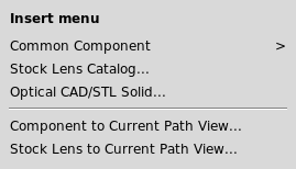
Use Insert for adding optics to the current design without replacing the active layout settings.

Insertion point

The table uses the current selection as the insertion anchor:

• If one or more rows are selected, inserted rows go below the last selected row.

• If the selected row belongs to a grouped element, selecting the # column selects the whole element block.

• If no row is selected, inserted rows go before the final Image row.

• Object and Image stay anchored and are not treated as component rows.

Surface and element clipboard

The table supports component-aware clipboard operations:

• Ctrl-C copies selected surface rows.

• If any selected row is part of a grouped element, the complete contiguous element block is copied.

• Ctrl-V pastes copied rows below the current selection.

• Object and Image are skipped on copy/paste.

• Pasted grouped elements receive independent element labels, so later Move Up/Down, Flip, Ungroup, and path assignment act on the pasted component rather than merging it with the source component.

The same commands are also available from Edit and from the table right-click menu.

Surface right-click menu

Right-clicking the Surface cell no longer opens only the type chooser. The same full menu is available from any table cell:

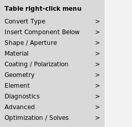
The table right-click menu groups row conversion, component insertion, geometry, diagnostics, and optimization actions.

• Convert Type changes the row to Standard, Aperture, Mirror, Object Target, Diffuse Object, Beam Splitter, Thin Lens, Grating, Image, or converts the selected physical row to an Optical CAD/STL Solid.

• Insert Component Below splices singlets, doublets, flat mirrors, object-target proxy rows, diffuse-object rows, plate/window rows, wedge prism rows, a right-angle prism primitive, a cube beam-splitter primitive, stock lenses, CAD/STL solids, or path-local components.

• Shape / Aperture exposes Shape Builder plus circular, rectangular, polygon/UDA, annulus, spider, and rectangular clear-aperture presets.

• Material opens the glass catalog and applies common materials to selected rows.

• Coating / Polarization opens coating/material editing, applies coating presets, enables metal Fresnel mirror mode, and configures beam-splitter Fresnel P/S behavior.

• Geometry aligns the local row orientation, sets TiltX incidence, reverses elements, and assigns/places rows on the current Path view.

• Element contains grouping, copy/paste, move, path assignment, and path role commands.

• Diagnostics sets trace/analysis targets and opens ray/path/scene inspectors.

• Advanced opens native KrakenOS attributes, Error Map, Grating/Galvo settings, and STL diagnostics/placement.

Compact prescription columns

The visible table keeps the columns that are edited most often during lens and layout work: surface type, material, radius, thickness, aperture, tilt, decenter, and axis movement. KrakenOS fields that are real but uncommon are kept in the row model and file export, but edited through Advanced....

k is the conic constant of the base sag. k = 0 is spherical, k = -1 is parabolic, values below -1 are hyperbolic, and positive values are oblate ellipsoids. Use it for conic/aspheric surfaces; ordinary spherical singlets and doublets usually leave it at zero.

Axicon is a conical sag angle in degrees. It is useful for axicons and Bessel-beam style layouts, but it is not a common day-to-day lens prescription field.

Open Advanced... -> Shape Params to edit either value. k can also be marked as an optimization variable from that pane; this writes KrakenOS-native Var/VarBounds metadata while keeping the main table compact.

Optimization cell marker

Cells selected as optimization variables use a Zemax-style split-cell marker: the main cell area keeps the numeric value, and a small right-side V badge marks that value as variable. This replaces the older * suffix and avoids coloring the whole row, so grouped element colors and row-selection borders remain readable.

Right-click a supported numeric cell and use Optimization / Solves -> Select ... for optimization. Supported visible variables include radius, thickness, tilt, decenter, and grating pitch. Hidden advanced variables such as conic k can still be enabled from their specialized dialog, but they do not reappear as main table columns.

The Optimization panel also has a Check Backend button. Use it before a long solve to confirm that the active Python environment can import pygmo, which is the global optimizer backend used by the UI. Start Optimization runs the same preflight automatically and aborts before spawning the worker if pygmo is missing; in the devenv workflow, run devenv shell kraken-install to reinstall the expected optimizer dependency set. Developer builds that need a non-wheel pagmo2 library can set KRAKEN_PAGMO2_LIB to the shared-library path, or to auto for the historical ~/Projects/pagmo2/_install/lib64/libpagmo.so location. For a command-line smoke test of the same backend and spawned-worker path, run python -m KrakenOS.UI.validate_optimization_backend.

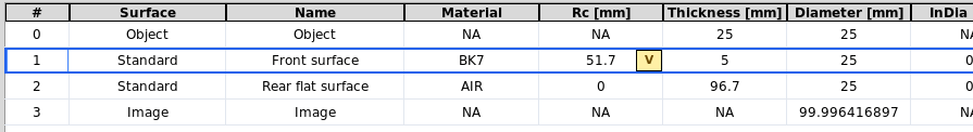
The V marker appears inside the selected numeric cell without replacing the row or element color.

Tolerance Monte Carlo report

The same variable markers can drive a manufacturing/tolerance sweep. Use Actions -> Tolerance Monte Carlo Report... after marking variables and choosing merit operands. The report samples each marked variable uniformly inside its current bounds, evaluates the selected merit function for every sample, and leaves the nominal editable table unchanged.

If no merit operand is selected, the report uses Spot RMS as the default diagnostic. The report is copied to the clipboard and written to Debug; use Actions -> Export Tolerance Monte Carlo CSV... to export the nominal row, each sampled variable value, total merit, operand values, residuals, and weighted contributions. This Phase 7E workflow is a deterministic batch engine and report schema.

By default, every marked tolerance variable is also a compensator. To model a manufacturing error that should be sampled but not adjusted during compensation, right-click the marked variable cell and choose Optimization / Solves -> Do not use ... as tolerance compensator. The UI saves this as row advanced ToleranceCompensators metadata. Scripts can make the same choice with set_tolerance_compensator_enabled(surface_index, parameter, enabled).

Manufacturing variables that move together can share one sampled degree of freedom. Right-click a marked variable cell and choose Optimization / Solves -> Set tolerance coupling group.... Variables with the same group name use the same random quantile during Monte Carlo. Prefix the group with - to make the variable move in the opposite direction, for example shared_mount on conic k and -shared_mount on TiltX. The UI saves this as row advanced ToleranceCoupling metadata. Scripts use set_tolerance_coupling(surface_index, parameter, group, sign=1) or sign=-1 for opposed motion.

Each tolerance variable can also carry named manufacturing metadata. Right-click the marked variable cell and choose Optimization / Solves -> Set manufacturing metadata.... Enter source type | source/spec ID | tags | note. For example, machined mount | MNT-001 | cell, vendor-a | shared cell machining attaches the variable to a named process/specification without changing how it is sampled. The UI saves this as row advanced ToleranceManufacturing metadata. Scripts use set_tolerance_manufacturing_metadata(surface_index, parameter, source_type=..., source_id=..., tags=(...), note=...). When the same source is reused, right-click a marked variable that already has metadata and choose Save manufacturing as template.... Other marked variables can then use Apply manufacturing template.... Templates are saved in the layout settings as tolerance_manufacturing_templates. Scripts use add_tolerance_manufacturing_template(name, source_type=..., source_id=..., tags=(...), note=...) and apply_tolerance_manufacturing_template(surface_index, parameter, template_or_name). Reports, presets, and CSV exports carry manufacturing_source_type, manufacturing_source_id, manufacturing_tags, and manufacturing_note columns.

After a Monte Carlo run, use Actions -> Tolerance Worst-Sample Comparison... to compare the nominal system against the worst valid perturbed sample. The comparison reports variable deltas, total-merit delta, and operand value/residual/weighted-term deltas. Actions -> Export Tolerance Comparison CSV... writes the same comparison records for external review.

Actions -> Tolerance Stack-Up Dashboard... ranks sampled tolerance variables using a linearized merit-variance proxy from the valid Monte Carlo samples. The report includes each variable’s merit slope, correlation, estimated contribution, worst-sample delta, and compensator/tolerance-only role. It also includes manufacturing-group rows: uncoupled variables become one-member groups, while ToleranceCoupling members are ranked together using the covariance of their sampled deltas. Named manufacturing source/type/tag/note metadata is copied into both the per-variable and group rows. This is a fast engineering dashboard, not a full Sobol decomposition. Use Actions -> Export Tolerance Stack-Up CSV... to export the per-variable ranked rows. Scripts can export the group rows with tolerance_stackup_group_csv_rows(dashboard).

Actions -> Tolerance Compensator Sweep... holds the temporary system at the worst valid Monte Carlo sample and sweeps each eligible compensator over its bounds. Actions -> Tolerance Multi-Compensator Solve... repeats bounded one-variable sweeps as a deterministic coordinate solve, accepting only merit-improving updates. Both reports are diagnostic and leave the nominal table unchanged; export their traces with the corresponding CSV actions.

Use Actions -> Save Tolerance Solve Preset... to persist the current Monte Carlo sample count, seed, compensator sweep steps, multi-compensator steps/passes, selected merit operands, TolCmp view, and tolerance-only versus compensator roles, coupling groups, and manufacturing metadata into the layout file. Actions -> Apply Tolerance Solve Preset... restores those choices without running a trace; the next tolerance report dialogs use the active preset as their initial defaults.

To see the effect geometrically, click the TolCmp analysis button and then Update after running the Monte Carlo report. The Tolerance compare left panel selector chooses the diagnostic:

Spot overlay

Overlays the nominal image-plane spot samples against the worst valid Monte Carlo sample, marks both centroids, and reports the merit and RMS spot-radius change.

Stack-up bars

Plots the covariance-aware manufacturing-group contribution rows from the tolerance stack-up dashboard. Coupled groups are shown as single bars, so a shared mount, spacer, or machining error is not visually double-counted.

MTF overlay

Rebuilds the same nominal/worst systems and plots their geometric MTF curves for the largest configured field sample. The annotation reports the selected tangential, sagittal, or average MTF value at the current MTF reference frequency.

Wavefront delta

Computes piston/tilt-removed WFE samples for the nominal and worst systems, then plots the centered worst - nominal wavefront delta over the pupil. The annotation reports nominal/worst WFE RMS plus delta RMS and P-V in waves.

Both overlays are diagnostic only: they rebuild temporary nominal/worst systems from the Monte Carlo records and do not change the editable table. Use Actions -> Export Tolerance Overlay CSV... to write the currently selected overlay data. The CSV schema follows the selected view: spot point coordinates, manufacturing-group stack-up rows, MTF frequency samples, or WFE pupil samples.

Prisms and cube beam splitters

Simple prisms can be built from table rows. A wedge prism is two tilted Standard surfaces: the first enters glass, the second exits to AIR. The right-click Insert Component Below -> Wedge Prism command creates this starter block.

For arbitrary prism solids, use Convert Type -> Optical CAD/STL Solid or Insert Component Below -> Optical CAD/STL Solid. A closed mesh is the physically correct UI representation when rays may hit side faces, experience total internal reflection, or leave through a non-sequential face.

After importing a file-backed solid, use Actions -> Assign CAD/STL Optical Faces or the row context menu Advanced -> Assign CAD/STL Optical Faces to record the optical intent of the mesh. The dialog clusters planar STL triangles into candidate faces and lets you assign Input Port / optional Output Port / Interaction Surface plus a coating model such as Uncoated, Full Reflecting, Partial Reflecting / Transmitting, or Absorbing / Mechanical. These labels are metadata used by the UI workflow and validators; KrakenOS still performs the physical ray trace through the closed Solid_3d_stl geometry and row material.

This is not yet the final prism authoring workflow. It is accurate as a KrakenOS execution model, but too pose-math-heavy for practical optical design. The future workflow should be a 3D scene-object placement tool: import the solid, select or fit the intended optical faces/axes visually, snap the prism to a traced ray or path frame, and then write the resulting pose back to the table only as saved implementation data.

Insert Component Below -> Cube Beam Splitter creates a practical starter: entrance face, internal 45 degree Beam Splitter surface, and transmit exit face. It is enough to start deterministic transmitted/reflected path design. For a closed cube with every side face available to tracing, use an Optical CAD/STL Solid for the external cube boundary and keep a Beam Splitter table surface for the internal coating/path metadata. Vendor CAD generally does not encode the split ratio, phase, or internal coating as ray-trace-ready physics.

Tilt and decenter tolerance overlays

The pose columns TiltX, TiltY, TiltZ, DespX, DespY, and DespZ accept comma-separated values or start:stop:step ranges. For example, enter -0.1, 0, 0.1 in TiltY or -0.05:0.05:0.05 in DespX.

The middle value becomes the nominal scalar KrakenOS row value. The full list is stored as Advanced -> Display2D -> pose_tolerance_overlay and the 2-D plot draws additional dashed ray traces plus dashed affected surface positions. If several pose cells contain lists with the same length, the values are swept together by index. If the list lengths differ, combinations are generated and truncated to 25 variants.

For grouped elements, enter the pose list once on any row in the element. The UI applies the same delta sweep to every row in the contiguous element block, so a doublet behaves like one mechanically shifted component instead of three independent tilted/decentered surfaces.

Mirror TiltX keeps the dedicated galvo/folded-scan interpretation because its displayed value is mirror slant, not raw KrakenOS local tilt. It still uses the same comma/range entry syntax.

Validation

Run the workflow regression check with:

python -m KrakenOS.UI.validate_table_component_workflow
python -m KrakenOS.UI.validate_compact_shape_fields

The first check inserts a common component while preserving global source/field settings, then copies and pastes grouped component rows while confirming that Object and Image are not duplicated. The compact-shape check confirms that k and Axicon are hidden from the main table, still reach KrakenOS surface construction, and remain optimizer-addressable where supported.