PupilCalc Tool

This page is a faithful conversion of Section 5 of the provisional manual (KrakenOS/Docs/USER_MANUAL_KrakenOS_Provisional.pdf, pages 21–27).

The system aperture — commonly the aperture stop (Ref. 5, §6.2) — is the element that defines how much light passes through the optical system. The image of the aperture formed by all elements in front of it is the entrance pupil; the image of the entrance pupil formed by the whole system is the exit pupil. The entrance pupil is not necessarily defined by the first element: sometimes it is set by a mechanical element rather than an optical surface.

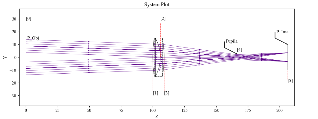
Figure 4. Visualization of two beams that coincide at the position defined as the pupil. (See appendix 7.10 — Examp_Doublet_Lens_Pupil.py.)

In the example above, the aperture stop sits on surface 4. Two beam fans arrive at field angles of +2° and −2°; their rays are collimated and pass together through the stop.

Tracing rays uniformly across the pupil one-by-one is awkward — fields with different origins on the object plane each need their own ray-direction calculations. PupilCalc automates that by sampling the pupil for a given field and aperture definition.

Code 5 — creating a PupilCalc object

W = 0.4
Surf = 4
AperVal = 10
AperType = "EPD"
Pup = Kos.PupilCalc(Doublet, Surf, W, AperType, AperVal)

Constructor arguments:

• Doublet — the optical system built from Kos.system

• Surf — index of the aperture-stop surface (surface 4 in Figure 4)

• W — wavelength at which the entrance and exit pupils are evaluated

• AperType — "STOP" (Surf is the aperture stop) or "EPD" (AperVal is the entrance-pupil diameter)

• AperVal — aperture-stop diameter or entrance-pupil diameter, depending on AperType

Pupil parameters

After construction, the resulting object exposes the pupil parameters:

Table 4 — pupil parameters on the PupilCalc object

Attribute	Meaning
Pup.RadPupInp	Entrance-pupil radius.
Pup.PosPupInp	Entrance-pupil position.
Pup.RadPupOut	Exit-pupil radius.
Pup.PosPupOut	Exit-pupil position.
Pup.PosPupOutFoc	Exit-pupil position relative to the focal plane.
Pup.DirPupSal	Exit-pupil orientation.

The pupil position is computed even when surfaces are decentered or tilted — in that case the displaced pupil becomes relevant when computing aberrations.

Automatic ray generation

PupilCalc also generates rays that uniformly sample the real pupil. The sampling is configured through the attributes below.

Table 5 — automatic ray generation from the pupil

Attribute	Meaning
Pup.Samp = #	Integer pupil-sampling parameter. Default 5.
Pup.Ptype = "<pattern>"	Pupil pattern. Allowed values: "rtheta" — one ray at radius Pup.rad (0–1) and angle Pup.theta (0–360°) on the unit pupil. "chief" — chief ray through the pupil centre. "hexapolar" — hexapolar pattern. "square" — rectangular grid. "fanx" — linear fan on the x-axis only. "fany" — linear fan on the y-axis only. "fan" — fans on both x and y. "rand" — random sampling.
Pup.FieldType = "height" or "angle"	Field type. "height" is used when the object is at a finite distance (object height in millimetres); "angle" is used when the rays arrive from infinity (degrees).
Pup.FieldX = # Pup.FieldY = #	Field value on the X and Y axes, in millimetres or degrees as set by FieldType.

To convert the unit-pupil sampling into real-world origins and direction cosines:

x, y, z, L, M, N = Pup.Pattern2Field()

x, y, z are the origin coordinates and L, M, N the direction cosines. The arrays can be iterated to trace each ray:

Code 6 — looped trace from a PupilCalc pattern

for i in range(0, len(x)):
    pSource_0 = [x[i], y[i], z[i]]
    dCos = [L[i], M[i], N[i]]
    Doublet.Trace(pSource_0, dCos, W)
    Rays.push()

The ray origins themselves can also be plotted. A hexapolar pattern is shown below.

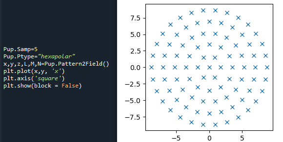
Figure 5. Generated code and pattern for the ray origins with a hexapolar distribution.

And the corresponding spot diagram at a 2° field:

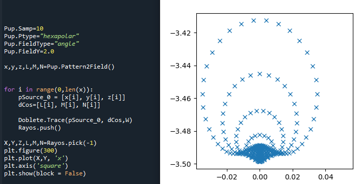
Figure 6. Code and spot diagram generated with a hexapolar pattern and a field angle of 2°.

When analyzing several fields, build a fresh pattern for each one and store the traces in separate Raykeeper containers to keep the results from mixing.

5.1 Atmospheric refraction in PupilCalc

When FieldType is "angle" — appropriate for telescopes, where rays arrive from infinity — PupilCalc can apply an atmospheric-refraction correction by deferring to the open-source AstroAtmosphere library (Ref. 3).

AstroAtmosphere computes the ray deviation from the observatory’s physical parameters: geographic latitude (deg), site altitude (m), humidity, CO₂ content (ppm), reference wavelength and zenith distance (deg). The settings below configure PupilCalc to apply that correction.

Code 7 — enabling atmospheric refraction

Pup.AtmosRef = 1       # 0 to disable, 1 to enable
Pup.T  = 283.15        # Temperature (K)
Pup.P  = 101300        # Atmospheric pressure (Pa)
Pup.H  = 0.5           # Humidity (0 to 1)
Pup.xc = 400           # CO2 (ppm)
Pup.lat = 31           # Latitude (degrees)
Pup.h  = 2800          # Observatory altitude (m)
Pup.l1 = 0.60169       # Reference wavelength (µm)
Pup.l2 = 0.50169       # Wavelength of interest (µm)
Pup.z0 = 55.0          # Zenith distance (degrees)

The example below generates three groups of rays for the same telescope at three different wavelengths:

Code 8 — building three wavelength groups

W1 = 0.50169
Pup.l2 = W1
xa, ya, za, La, Ma, Na = Pup.Pattern2Field()

W2 = 0.60169
Pup.l2 = W2
xb, yb, zb, Lb, Mb, Nb = Pup.Pattern2Field()

W3 = 0.70169
Pup.l2 = W3
xc, yc, zc, Lc, Mc, Nc = Pup.Pattern2Field()

Each group is traced and pushed into its own Raykeeper:

Code 9 — tracing each wavelength group

for i in range(0, len(xa)):
    Telescope.Trace([xa[i], ya[i], za[i]], [La[i], Ma[i], Na[i]], W1)
    Rays1.push()

for i in range(0, len(xb)):
    Telescope.Trace([xb[i], yb[i], zb[i]], [Lb[i], Mb[i], Nb[i]], W2)
    Rays2.push()

for i in range(0, len(xc)):
    Telescope.Trace([xc[i], yc[i], zc[i]], [Lc[i], Mc[i], Nc[i]], W3)
    Rays3.push()

Plotting the per-wavelength spot diagrams shows a separation of roughly 72 µm between the extreme wavelengths (blue and green crosses in Figure 7):

Code 10 — plotting the per-wavelength spot diagrams

X, Y, Z, L, M, N = Rays1.pick(-1)
plt.plot(X * 1000.0, Y * 1000.0, 'x', c="b")

X, Y, Z, L, M, N = Rays2.pick(-1)
plt.plot(X * 1000.0, Y * 1000.0, 'x', c="r")

X, Y, Z, L, M, N = Rays3.pick(-1)
plt.plot(X * 1000.0, Y * 1000.0, 'x', c="g")

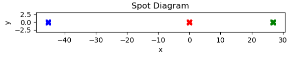
Figure 7. Images formed by a telescope that are spectrally displaced by the action of atmospheric refraction.