Chapter 4: Geometrical Optics
Source: Eugene Hecht, Schaum’s Outline of Theory and Problems of Optics (1975), Chapter 4. The entries below cover only the chapter’s Supplementary Problems; prompts are paraphrased and are not reproduced.
Each numbered solution states its assumptions, develops the algebra, substitutes the relevant data, and checks the result. Original SVG illustrations show the ray geometry, field relationships, or calculated curves. Diagrams are schematic unless their axes specify a scale. Source inconsistencies and approximations are identified explicitly rather than silently copied into the answer.
Aspherical refracting surfaces
Formula and definitions.
Fermat’s principle requires the optical path from the object wavefront to the image point to be independent of aperture coordinate. Write both Euclidean distances, multiply by their indices, evaluate the constant at the vertex, and square only after isolating one radical. Completing the square identifies the conic and its eccentricity.
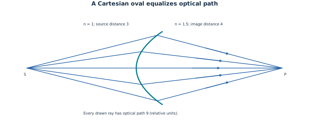
Equal optical paths define a Cartesian oval. The plotted interface focuses a real axial source into a second medium.
Problem 4.62 — derive the Cartesian-ovoid equation in vertex coordinates
Paraphrased task. Derive the cartesian-ovoid equation in vertex coordinates.
Formula reference. Use (1), its definitions, and the topic illustration.
Worked application.
Put the vertex at \((0,0)\), a real source at \((-s_o,0)\), and the desired real image at \((s_i,0)\). Here \(s_o,s_i>0\) are geometric distances, not signed Cartesian coordinates.
For a surface point \(Q=(x,y)\), Pythagoras gives \(SQ=\sqrt{(x+s_o)^2+y^2}\) and \(QP=\sqrt{(s_i-x)^2+y^2}\). Multiply each length by its medium’s index.
Equal optical path through every surface point, including the vertex, requires
\[n_i\sqrt{(x+s_o)^2+y^2}+n_t\sqrt{(s_i-x)^2+y^2} =n_is_o+n_ts_i.\]This implicit curve is the Cartesian oval. Rotation about the source-image axis gives the refracting surface; differentiating its constant optical path gives Snell’s law.
Result. The weighted-distance equation above defines the stigmatic interface.
Check. Setting \(x=y=0\) recovers the vertex optical path. Virtual endpoints require signed optical lengths rather than blindly reusing positive distances.
Problem 4.63 — prove that a plane-wave focusing surface is an ellipsoid
Paraphrased task. Prove that a plane-wave focusing surface is an ellipsoid.
Formula reference. Use (1), its definitions, and the topic illustration.
Worked application.
A plane wave travelling along \(+x\) reaches the surface point \((x,y)\) after an extra incident optical distance \(n_ix\). Equal path to the focus \((s_i,0)\) requires \(n_ix+n_t\sqrt{(s_i-x)^2+y^2}=n_ts_i\).
Isolate the square root, square, and collect terms:
\[(n_t^2-n_i^2)x^2-2n_ts_i(n_t-n_i)x+n_t^2y^2=0.\]For \(n_t>n_i\), divide by \(n_t^2-n_i^2\) and complete the square. With \(a=n_ts_i/(n_t+n_i)\) and \(b=s_i\sqrt{(n_t-n_i)/(n_t+n_i)}\), the equation is \((x-a)^2/a^2+y^2/b^2=1\). Consequently \(e=\sqrt{1-b^2/a^2}=n_i/n_t\).
Result. An ellipsoid of revolution, with \(a=n_ts_i/(n_t+n_i)\), \(b=s_i\sqrt{(n_t-n_i)/(n_t+n_i)}\), and \(e=n_i/n_t\).
Check. Retain only the branch satisfying the unsquared optical-path equation; squaring alone can introduce an unphysical branch.
Problem 4.64 — prove that a plane-wave diverging surface is a hyperboloid
Paraphrased task. Prove that a plane-wave diverging surface is a hyperboloid.
Formula reference. Use (1), its definitions, and the topic illustration.
Worked application.
The apparent focus lies at \(s_i<0\). For a diverging transmitted wave, subtract its distance to the virtual focus: \(n_ix-n_t\sqrt{(x-s_i)^2+y^2}=n_ts_i\).
Squaring gives the same polynomial as in Problem 4.63. Now \(n_i>n_t\), so the coefficients of \(x^2\) and \(y^2\) have opposite signs.
Define \(a=|n_ts_i|/(n_i+n_t)\), \(b=|s_i|\sqrt{(n_i-n_t)/(n_i+n_t)}\), and \(x_c=n_ts_i/(n_i+n_t)\). Completing the square gives
\[\frac{(x-x_c)^2}{a^2}-\frac{y^2}{b^2}=1, \qquad e=\sqrt{1+b^2/a^2}=\frac{n_i}{n_t}>1.\]Choose the sheet passing through the vertex and satisfying the unsquared equation.
Result. A hyperboloid of revolution with eccentricity \(n_i/n_t\) and a virtual focus at \(P\).
Check. The change from ellipse to hyperbola follows from the sign of \(n_t^2-n_i^2\), not from a change in Snell’s law.
Spherical refracting surfaces
Formula and definitions.
Adopt the Cartesian sign convention printed in the chapter: real incident objects have positive \(s_o\), and the sign of \(R\) follows the center of curvature. Solve the surface equation before applying magnification. A point at the center of curvature is undeviated.
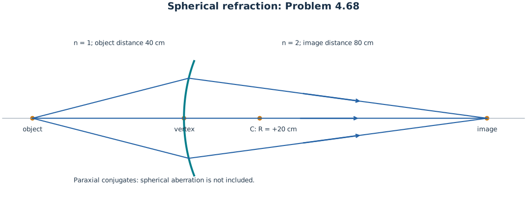
Spherical-interface conjugates depend on the incident and transmitted indices and the signed radius of curvature.
Problem 4.65 — locate a flaw imaged through a hemispherical diamond end
Paraphrased task. Locate a flaw imaged through a hemispherical diamond end.
Formula reference. Use (2), its definitions, and the topic illustration.
Worked application.
Orient the axis along light leaving the diamond. The flaw is at the centre of curvature, so \(s_o=20\,\mathrm{cm}\) and \(R=-20\,\mathrm{cm}\).
Apply the spherical-interface equation with \(n_i=2.42\), \(n_t=1.33\):
\[\frac{2.42}{20}+\frac{1.33}{s_i} =\frac{1.33-2.42}{-20}=0.0545, \qquad s_i=-20\,\mathrm{cm}.\]All rays from the centre strike the sphere normally and therefore keep their directions. Their backward extensions still meet at the original flaw, giving a virtual image there.
Result. \(s_i=-20\,\mathrm{cm}\); the image coincides with the flaw.
Check. The geometric normal-incidence argument is exact, not merely paraxial, and is independent of the surrounding refractive index.
Problem 4.66 — place a source for a spherical-plus-hyperboloidal glass rod
Paraphrased task. Place a source for a spherical-plus-hyperboloidal glass rod.
Formula reference. Use (2), its definitions, and the topic illustration.
Worked application.
The right hyperboloid has \(e=n_{\rm glass}/n_{\rm air}=1.5\). Its specified virtual focus is therefore the image of a collimated beam travelling inside the rod.
The left hemisphere has \(R=5\,\mathrm{cm}\). Demand \(s_i\to\infty\) at this first air-glass interface:
\[\frac{1}{s_o}+\frac{1.5}{\infty} =\frac{1.5-1}{5},\qquad s_o=10\,\mathrm{cm}.\]Put the source at this object focal point. Refraction at the hemisphere produces the paraxial parallel bundle; the hyperboloid then makes it appear to diverge from its first focus, 5 cm left of its vertex.
Result. Place the source \(10\,\mathrm{cm}\) to the left of the spherical vertex.
Check. The spherical entrance is only paraxially collimating; a finite-aperture spherical entrance still has spherical aberration.
Problem 4.67 — image an ant through a glass sphere in alcohol
Paraphrased task. Image an ant through a glass sphere in alcohol.
Formula reference. Use (2), its definitions, and the topic illustration.
Worked application.
At the near surface, the ant is \(s_o=6-4=2\,\mathrm{cm}\) from the vertex. The centre is on the transmitted side, hence \(R=+4\,\mathrm{cm}\).
Use alcohol as the incident medium and glass as the transmitted medium:
\[\frac{1.36}{2}+\frac{1.50}{s_i} =\frac{1.50-1.36}{4}=0.035, \qquad s_i=\frac{1.50}{-0.645}=-2.326\,\mathrm{cm}.\]The transverse magnification of a refracting surface is \(M_T=-n_is_i/(n_ts_o)=1.054\). The first-surface image is virtual, upright, and slightly enlarged.
Result. The near interface forms a virtual image \(2.33\,\mathrm{cm}\) outside its vertex, with \(M_T\approx1.05\).
Check. This is the image formed by the first interface. Observing through the entire sphere would require a second refraction.
Problem 4.68 — infer the radius of a convex refracting interface
Paraphrased task. Infer the radius of a convex refracting interface.
Formula reference. Use (2), its definitions, and the topic illustration.
Worked application.
The real object and image give \(s_o=40\,\mathrm{cm}\), \(s_i=80\,\mathrm{cm}\), with \(n_i=1\), \(n_t=2\).
Rearrange the surface equation to isolate curvature:
\[R=\frac{n_t-n_i}{n_i/s_o+n_t/s_i} =\frac{1}{1/40+2/80}=20\,\mathrm{cm}.\]The positive sign places the centre of curvature in the second medium; this is a convex entrance surface as seen by the incident rays.
Result. \(R=+20\,\mathrm{cm}\).
Check. Both terms on the left of the conjugate equation are positive, consistent with a positive refracting power.
Thin-lens equation and imagery
Formula and definitions.
Use the lensmaker equation only to obtain \(f\); use the Gaussian thin-lens equation for conjugates. Combine \(s_i=-M_Ts_o\) with either \(s_o+s_i=L\) or the specified separation to remove one unknown. The two Bessel locations arise from the quadratic in \(s_o\).
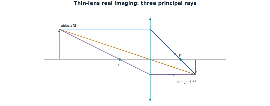
A positive thin lens forms a real inverted image when the object is outside its front focal point.
Problem 4.69 — relate an unequal biconvex lens radius to focal length
Paraphrased task. Relate an unequal biconvex lens radius to focal length.
Formula reference. Use (3), its definitions, and the topic illustration.
Worked application.
Let the smaller radius magnitude be \(R\). A double-convex lens has opposite signed radii; take \(R_1=2R\), \(R_2=-R\).
The thin-lens maker equation in air is
\[\frac1f=(1.5-1)\left(\frac1{2R}-\frac1{-R}\right) =\frac{3}{4R}.\]Multiply by \(fR\) to obtain \(R=3f/4\). Reversing the lens interchanges the magnitudes but leaves its thin-lens power unchanged.
Result. The smaller radius magnitude is \(3f/4\); the larger is \(3f/2\).
Check. Using two positive signed radii would describe a meniscus, not the specified biconvex lens.
Problem 4.70 — derive the two Bessel positions of a lens between object and screen
Paraphrased task. Derive the two bessel positions of a lens between object and screen.
Formula reference. Use (3), its definitions, and the topic illustration.
Worked application.
If the lens is \(s\) from the source, its distance to the screen is \(L-s\). Real imaging requires \(0<s<L\).
Substitute in the thin-lens equation: \(1/f=1/s+1/(L-s)=L/[s(L-s)]\). Thus \(s^2-Ls+fL=0\).
Solve the quadratic:
\[s_\pm=\frac{L\pm\sqrt{L(L-4f)}}2.\]Two different positions exist for \(L>4f\); they merge at \(s=2f\) for \(L=4f\). No real lens placement works for \(L<4f\).
Result. \(s_\pm=[L\pm\sqrt{L(L-4f)}]/2\).
Check. The two roots sum to \(L\), so exchanging the object and image distances exchanges the two positions.
Problem 4.71 — find the radii of an equiconvex flint lens
Paraphrased task. Find the radii of an equiconvex flint lens.
Formula reference. Use (3), its definitions, and the topic illustration.
Worked application.
An equiconvex lens has \(R_1=R\), \(R_2=-R\) in the left-to-right sign convention.
With \(n=1.65\), the lens maker equation becomes \(1/f=0.65(2/R)=1.30/R\).
For \(f=62\,\mathrm{cm}\), \(R=1.30(62)=80.6\,\mathrm{cm}\). Assign the signs only after calculating the common magnitude.
Result. \(R_1=+80.6\,\mathrm{cm}\), \(R_2=-80.6\,\mathrm{cm}\).
Check. Substitution gives \(0.65(1/80.6+1/80.6)=1/62\,\mathrm{cm}^{-1}\).
Problem 4.72 — image a converging bundle through a negative lens
Paraphrased task. Image a converging bundle through a negative lens.
Formula reference. Use (3), its definitions, and the topic illustration.
Worked application.
A converging incident bundle has a virtual object on the transmitted side. Write \(s_o=-a\) with \(a>0\); write the negative lens focal length as \(f=-F\), \(F>0\).
The lens equation gives
\[-\frac1F=-\frac1a+\frac1{s_i},\qquad s_i=\frac{aF}{F-a}.\]If \(a<F\), then \(s_i>0\) and \(s_i/a=F/(F-a)>1\). Also \(M_T=-s_i/s_o=F/(F-a)>1\). The lens weakens the convergence, so the focus moves farther away but remains real.
Result. For \(|s_o|<|f|\), the image is real, erect relative to the virtual object, and enlarged.
Check. At \(a=F\) the emerging light is parallel; for \(a>F\) it diverges and the image is virtual.
Problem 4.73 — design a slide-projector conjugate
Paraphrased task. Design a slide-projector conjugate.
Formula reference. Use (3), its definitions, and the topic illustration.
Worked application.
The requested scale factor is \(2000/20=3000/30=100\). A real projected image is inverted, so \(M_T=-100\).
With the wall \(s_i=10\,\mathrm m\) from the lens, \(M_T=-s_i/s_o\) gives \(s_o=10/100=0.10\,\mathrm m\).
Calculate the focal length without rounding the reciprocal terms:
\[f=\frac{s_os_i}{s_o+s_i} =\frac{0.10(10)}{10.10}=0.09901\,\mathrm m.\]
Result. Place the slide \(10\,\mathrm{cm}\) from a lens with \(f\approx99.0\,\mathrm{mm}\).
Check. The slide is just beyond the front focal plane, as required for a large real projection.
Problem 4.74 — find a lens making an erect enlarged image
Paraphrased task. Find a lens making an erect enlarged image.
Formula reference. Use (3), its definitions, and the topic illustration.
Worked application.
The image is erect, so its signed magnification is \(M_T=8/5=+1.6\).
With a real object \(s_o=90\,\mathrm{cm}\), \(s_i=-M_Ts_o=-144\,\mathrm{cm}\). The negative image distance means a virtual image on the object’s side.
Substitute both signed distances:
\[\frac1f=\frac1{90}-\frac1{144}=\frac1{240}, \qquad f=240\,\mathrm{cm}.\]
Result. \(f=240\,\mathrm{cm}\) and \(s_i=-144\,\mathrm{cm}\).
Check. \(s_o<f\), exactly the regime in which a positive lens forms an enlarged upright virtual image.
Problem 4.75 — solve camera object and film distances
Paraphrased task. Solve camera object and film distances.
Formula reference. Use (3), its definitions, and the topic illustration.
Worked application.
Convert the object height to millimetres: \(h_o=1000\,\mathrm{mm}\). The inverted film image has \(M_T=-25/1000=-0.025\), so \(s_i=0.025s_o\).
Substitute into \(1/50=1/s_o+1/(0.025s_o)=41/s_o\), obtaining \(s_o=2050\,\mathrm{mm}\).
The film separation is \(s_i=0.025(2050)=51.25\,\mathrm{mm}\). These values follow directly from the stated heights and focal length; slightly different endpoints printed in the scan do not satisfy both equations.
Result. Object-lens distance \(2.05\,\mathrm m\); lens-film distance \(51.25\,\mathrm{mm}\).
Check. \(1/2050+1/51.25=1/50\) and \(51.25/2050=0.025\).
Problem 4.76 — derive an object-image separation identity
Paraphrased task. Derive an object-image separation identity.
Formula reference. Use (3), its definitions, and the topic illustration.
Worked application.
Define the signed axial object-image separation \(L=s_o+s_i\), and use \(M_T=-s_i/s_o\).
The lens equation and \(s_i=-M_Ts_o\) give \(s_o=f(1-1/M_T)\) and \(s_i=f(1-M_T)\).
Add the two distances and simplify:
\[L=f\left(2-M_T-\frac1{M_T}\right) =-\frac{f(M_T-1)^2}{M_T}.\]For a real object and real image, \(M_T<0\) and this is their positive physical separation. Other configurations require the absolute coordinate separation if an unsigned distance is wanted.
Result. \(L=-f(M_T-1)^2/M_T\) under the stated signed convention.
Check. \(M_T=-1\) gives \(L=4f\), the minimum real-conjugate separation.
Compound thin lenses
Formula and definitions.
For separated lenses either multiply paraxial matrices or image sequentially. In sequential form, the first image position supplies the second object distance with the separation and sign handled explicitly. In matrix form, the equivalent power is \(-C\).
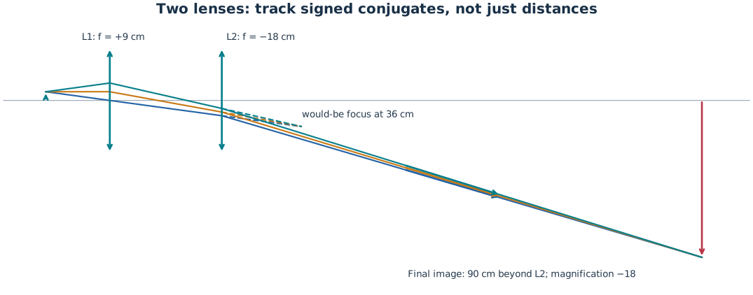
Sequential paraxial tracing for Problem 4.80: the second lens intercepts a converging bundle and moves its final focus farther away.
Problem 4.77 — obtain front and back focal lengths of a telephoto pair
Paraphrased task. Obtain front and back focal lengths of a telephoto pair.
Formula reference. Use (4), its definitions, and the topic illustration.
Worked application.
For separated thin lenses, \(\Phi=1/f_1+1/f_2-d/(f_1f_2)\). With \(f_1=20\), \(f_2=-40\), \(d=10\) cm, \(\Phi=0.0375\,\mathrm{cm}^{-1}\) and \(f=26.6667\,\mathrm{cm}\).
The system matrix has \(A=1-d/f_1=0.5\), \(D=1-d/f_2=1.25\), \(C=-\Phi\). The rear focal distance from lens 2 is \(-A/C=Af\).
The front focal distance to the left of lens 1 is \(-D/C=Df\). Thus \(\mathrm{BFL}=13.3333\,\mathrm{cm}\) and \(\mathrm{FFL}=33.3333\,\mathrm{cm}\).
Result. Front focus \(33.33\,\mathrm{cm}\) left of lens 1; rear focus \(13.33\,\mathrm{cm}\) right of lens 2.
Check. The total lens-1-to-rear-focus length is \(23.33\,\mathrm{cm}<f\), the characteristic telephoto shortening.
Problem 4.78 — combine three lenses in contact and locate an image
Paraphrased task. Combine three lenses in contact and locate an image.
Formula reference. Use (4), its definitions, and the topic illustration.
Worked application.
Lenses in contact add powers: \(1/f=1/10+1/20-1/40=1/8\), with lengths in centimetres.
For \(s_o=16\,\mathrm{cm}\), \(1/s_i=1/8-1/16=1/16\), giving \(s_i=16\,\mathrm{cm}\).
The magnification is \(M_T=-16/16=-1\). The image is real, inverted, and the same size as the object.
Result. \(f=8\,\mathrm{cm}\), \(s_i=16\,\mathrm{cm}\), \(M_T=-1\).
Check. An object at \(2f\) is imaged at \(2f\); the negative component reduces, but does not cancel, the positive total power.
Problem 4.79 — split a known contact-lens power in a two-to-one ratio
Paraphrased task. Split a known contact-lens power in a two-to-one ratio.
Formula reference. Use (4), its definitions, and the topic illustration.
Worked application.
Let the weaker lens power be \(P\) and the stronger be \(2P\). Contact placement makes the combined power \(3P\).
The combined focal length is \(30\,\mathrm{cm}=0.30\,\mathrm m\), so \(3P=1/0.30\) and \(P=1.1111\,\mathrm D\).
Invert each power: \(f_{\rm weak}=0.90\,\mathrm m\) and \(f_{\rm strong}=0.45\,\mathrm m\).
Result. The focal lengths are \(90\,\mathrm{cm}\) and \(45\,\mathrm{cm}\).
Check. Twice the power means half the focal length, not twice the focal length.
Problem 4.80 — propagate an image through two separated lenses
Paraphrased task. Propagate an image through two separated lenses.
Formula reference. Use (4), its definitions, and the topic illustration.
Worked application.
Lens 1 has \(f_1=9\,\mathrm{cm}\) and \(s_{o1}=12\,\mathrm{cm}\). Hence \(s_{i1}=(1/9-1/12)^{-1}=36\,\mathrm{cm}\).
Lens 2 is only 21 cm beyond lens 1. Its incident light is still converging to a point 15 cm beyond it, so \(s_{o2}=21-36=-15\,\mathrm{cm}\).
For \(f_2=-18\,\mathrm{cm}\),
\[\frac1{s_{i2}}=-\frac1{18}-\frac1{-15}=\frac1{90}.\]The component magnifications are \(M_1=-3\) and \(M_2=+6\); the total is \(M_T=-18\).
Result. The final image is real, \(90\,\mathrm{cm}\) right of lens 2, inverted and enlarged by a factor of 18.
Check. Assigning a positive object distance to the converging bundle at lens 2 would give the wrong image side.
Thick lenses
Formula and definitions.
Represent refraction by reduced-angle matrices and the internal thickness by translation in the lens index. Multiply in encounter order (rightmost matrix first), then read the effective focal length and principal plane offsets from \(A,C,D\). Image from the principal planes, not from the vertices.
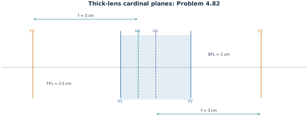
Problem 4.82: principal planes lie inside the thick lens, so effective and vertex focal distances are different.
Problem 4.81 — analyze an equal-negative-radius index-two thick lens
Paraphrased task. Analyze an equal-negative-radius index-two thick lens.
Formula reference. Use (5), its definitions, and the topic illustration.
Worked application.
For \(n=2\), \(R_1=R_2=R<0\), and thickness \(d\), the two surface powers cancel in the zero-thickness limit. The finite-thickness term remains:
\[\Phi=(n-1)\left(\frac1{R_1}-\frac1{R_2}\right) +\frac{(n-1)^2d}{nR_1R_2}=\frac{d}{2R^2}.\]Therefore \(f=1/\Phi=2R^2/d>0\). The centre separation equals the vertex separation because the signed radii are equal.
Principal-plane offsets, positive to the right of each corresponding vertex, are \(h_1=-f(n-1)d/(nR_2)=-R\) and \(h_2=-f(n-1)d/(nR_1)=-R\). Both planes shift right by \(|R|\) and remain separated by \(d\).
Result. A positive lens with \(f=2R^2/d\) and \(h_1=h_2=-R\).
Check. As \(d\to0\), the power tends to zero even though the limiting principal-plane offsets remain finite.
Problem 4.82 — locate principal and focal points of a thick biconvex lens
Paraphrased task. Locate principal and focal points of a thick biconvex lens.
Formula reference. Use (5), its definitions, and the topic illustration.
Worked application.
Use \(R_1=+2\), \(R_2=-4\), \(d=2\) cm and \(n=1.5\). The thick-lens power is \(\Phi=0.5(1/2+1/4)+0.25(2)/(1.5\cdot2\cdot(-4))=1/3\,\mathrm{cm}^{-1}\).
Thus \(f=3\,\mathrm{cm}\). The principal offsets are \(h_1=-3(0.5)(2)/(1.5(-4))=+0.5\,\mathrm{cm}\) and \(h_2=-3(0.5)(2)/(1.5(2))=-1\,\mathrm{cm}\).
Measure the front focus from vertex 1 as \(h_1-f=-2.5\,\mathrm{cm}\) and the rear focus from vertex 2 as \(h_2+f=+2\,\mathrm{cm}\). Effective focal length is measured from the principal planes, not from the glass vertices.
Result. \(H_1\) is 0.5 cm right of \(V_1\); \(H_2\) is 1 cm left of \(V_2\); front/rear vertex focal distances are 2.5 cm left and 2 cm right.
Check. The two principal planes lie inside this lens; neglecting the thickness term would incorrectly give \(f=2.667\,\mathrm{cm}\).
Problem 4.83 — image through a hemispherical thick lens
Paraphrased task. Image through a hemispherical thick lens.
Formula reference. Use (5), its definitions, and the topic illustration.
Worked application.
Take the curved face first: \(R_1=12\,\mathrm{cm}\), \(R_2=\infty\), \(d=12\,\mathrm{cm}\), \(n=2\). Only the curved surface contributes power, so \(f=R_1/(n-1)=12\,\mathrm{cm}\).
The principal offsets are \(h_1=0\) and \(h_2=-fd/(2R_1)=-6\,\mathrm{cm}\). The front focus is 12 cm left of the curved vertex; the rear focus is 6 cm beyond the plane face.
The object is \(s_o=36\,\mathrm{cm}\) from \(H_1\). Therefore \(s_i=(1/12-1/36)^{-1}=18\,\mathrm{cm}\) from \(H_2\), or 12 cm beyond the plane face. \(M_T=-18/36=-1/2\).
Result. A real, inverted, half-size image 18 cm right of \(H_2\), equivalently 12 cm beyond the plane face.
Check. The planar exit has zero surface power but shifts the rear principal plane; treating the hemisphere as a zero-thickness lens misplaces the image.
Problem 4.84 — analyze a common-center thick lens
Paraphrased task. Analyze a common-center thick lens.
Formula reference. Use (5), its definitions, and the topic illustration.
Worked application.
For the common centre to the left, let \(R_1=-a\), \(R_2=-(a+d)\), with \(a>0\). Both radius vectors point back to the same physical point.
With \(n=2\), collect the thick-lens terms:
\[\Phi=-\frac1a+\frac1{a+d}+\frac{d}{2a(a+d)} =-\frac{d}{2a(a+d)},\qquad f=-\frac{2a(a+d)}d.\]The offsets become \(h_1=-fd/(2R_2)=-a\) and \(h_2=-fd/(2R_1)=-(a+d)\). In global coordinates both locate the common centre, so the two principal planes coincide there.
Result. A negative lens with \(f=-2a(a+d)/d\); both principal planes pass through the common centre.
Check. The negative power follows from concave entrance power exceeding convex exit power; the thickness correction only partly cancels it.
Problem 4.85 — image with a spherical benzene droplet
Paraphrased task. Image with a spherical benzene droplet.
Formula reference. Use (5), its definitions, and the topic illustration.
Worked application.
A ball lens has \(R_1=r\), \(R_2=-r\), \(d=2r\). Its power reduces to \(\Phi=2(n-1)/(nr)\) and both principal planes pass through the centre.
For \(n=1.501\), \(r=2\,\mathrm{mm}\), \(f=nr/[2(n-1)]=2.9960\,\mathrm{mm}\). The object distance from the principal plane is \(s_o=58\,\mathrm{mm}\).
Compute \(s_i=fs_o/(s_o-f)=3.1592\,\mathrm{mm}\), \(M_T=-s_i/s_o=-0.05447\), and \(h_i=M_T(0.5)=-0.02723\,\mathrm{mm}\).
Result. The image is real, inverted, and about \(0.027\,\mathrm{mm}\) tall, \(3.16\,\mathrm{mm}\) from the droplet centre.
Check. The image is \(1.16\,\mathrm{mm}\) beyond the rear surface. The quoted rounded \(f\approx3\,\mathrm{mm}\) is consistent with this result.
Lens combinations
Formula and definitions.
Translate each focal length to a lens power and each spacing to a translation matrix. Multiplying the complete train exposes its cardinal points. A collimated input has zero reduced angle change only when the system element \(C\) vanishes.
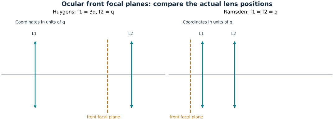
Huygens and Ramsden oculars have different front focal-plane positions despite both producing collimated output.
Problem 4.86 — locate the first focal plane of a Huygens ocular
Paraphrased task. Locate the first focal plane of a huygens ocular.
Formula reference. Use (6), its definitions, and the topic illustration.
Worked application.
Write the eye-lens focal length as \(q\). Then \(f_1=3q\), \(f_2=q\), \(d=2q\), so \(\Phi=1/(3q)+1/q-2/(3q)=2/(3q)\) and \(f=3q/2\).
The matrix entry \(D=1-d/f_2=-1\). The signed front focal distance to the left of lens 1 is \(Df=-3q/2\): the front focal plane is actually \(3q/2\) to its right.
Lens 2 is at \(2q\), so that plane is \(q/2\) left of the eye lens. The incident bundle must converge toward that plane; the ocular then converts it to parallel light.
Result. The first focal plane lies between the lenses, \(q/2\) before the eye lens; the effective focal length is \(3q/2\).
Check. The first principal plane is \(fd/f_2=3q\) right of lens 1, and its front focus is one effective focal length to its left.
Problem 4.87 — place an object for a two-lens image on a screen
Paraphrased task. Place an object for a two-lens image on a screen.
Formula reference. Use (6), its definitions, and the topic illustration.
Worked application.
Work backward from the required \(s_{i2}=45\,\mathrm{cm}\) and \(f_2=60\,\mathrm{cm}\): \(1/s_{o2}=1/60-1/45=-1/180\), so \(s_{o2}=-180\,\mathrm{cm}\).
This virtual object is 180 cm beyond lens 2, hence lens 1 must form its intermediate image \(s_{i1}=20+180=200\,\mathrm{cm}\) to its right.
With \(f_1=40\,\mathrm{cm}\), \(1/s_{o1}=1/40-1/200=1/50\). Therefore the source belongs 50 cm before lens 1. The total magnification is \((-200/50)(-45/(-180))=-1\).
Result. Place the object \(50\,\mathrm{cm}\) left of lens 1; its final real image is inverted and equal in size.
Check. The equivalent \(f=30\,\mathrm{cm}\) has principal-plane conjugates \(60\,\mathrm{cm}\) and \(60\,\mathrm{cm}\), confirming unit inverted magnification.
Problem 4.88 — choose the third focal length of an afocal triplet
Paraphrased task. Choose the third focal length of an afocal triplet.
Formula reference. Use (6), its definitions, and the topic illustration.
Worked application.
Trace a parallel paraxial ray of height \(h\) and slope zero. After lens 1, \(u_1=-h/4\); after propagation through 6 cm, \(y_2=h+6u_1=-h/2\).
The negative lens has \(f_2=-8\,\mathrm{cm}\). Its output slope is \(u_2=u_1-y_2/f_2=-h/4-h/16=-5h/16\). At lens 3, 1.4 cm later, \(y_3=-h/2-(1.4)(5h/16)=-15h/16\).
Afocality requires \(u_3=u_2-y_3/f_3=0\). Hence \(f_3=y_3/u_2=3\,\mathrm{cm}\). The arbitrary input height cancels, as it must for a first-order afocal system.
Result. \(f_3=+3.0\,\mathrm{cm}\).
Check. The last positive lens receives a diverging bundle from its front focal plane and collimates it.
Problem 4.89 — locate the object plane of a Ramsden ocular
Paraphrased task. Locate the object plane of a ramsden ocular.
Formula reference. Use (6), its definitions, and the topic illustration.
Worked application.
Let each lens have focal length \(q\), with separation \(d=2q/3\). The combined power is \(2/q-d/q^2=4/(3q)\), so \(f=3q/4\).
The front principal plane is \(h_1=fd/q=q/2\) to the right of the field lens. Its front focus is therefore at \(h_1-f=-q/4\) relative to that lens.
Place the object plane \(q/4\) before the field lens, equivalently \(3q/4\) before \(H_1\). Rays from this plane emerge collimated. The effective focal length alone is not the distance from the first glass element.
Result. The object plane is \(q/4\) in front of the first lens, or \(3q/4\) in front of the first principal plane.
Check. Sequentially, lens 1 gives \(s_{i1}=-q/3\); lens 2 then sees \(s_{o2}=2q/3+q/3=q\) and produces parallel light.
Problem 4.90 — verify an afocal positive-negative lens prescription
Paraphrased task. Verify an afocal positive-negative lens prescription.
Formula reference. Use (6), its definitions, and the topic illustration.
Worked application.
Use the intended positive power \(P_1=10/3\,\mathrm D\), negative power \(P_2=-20\,\mathrm D\), and separation \(d=1/4\,\mathrm m\).
Separated powers combine as
\[P=P_1+P_2-dP_1P_2 =\frac{10}{3}-20-\frac14\frac{10}{3}(-20)=0.\]Thus the focal length is infinite and a parallel input gives a parallel output. If the rounded value \(3.33\,\mathrm D\) is taken literally, \(P=-0.02\,\mathrm D\) and \(f=-50\,\mathrm m\), a nearly afocal system rather than exactly zero power.
Result. The intended system is afocal; exact cancellation uses \(P_1=3\frac13\,\mathrm D\).
Check. The separation equals \(f_1+f_2=0.30-0.05=0.25\,\mathrm m\), the telescope afocal condition.
Planar, aspherical, and spherical mirrors
Formula and definitions.
Reflection is reciprocal: exchanging a real object and real image leaves the mirror equation unchanged. For a virtual object use the signed negative \(s_o\) specified by the converging incident bundle. Magnification fixes orientation and height after the conjugates are known.
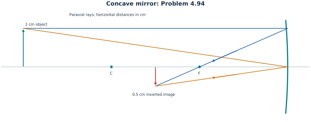
Problem 4.94: rays from the object meet at a real, inverted, half-height mirror image.
Problem 4.91 — exchange object and image locations for a concave mirror
Paraphrased task. Exchange object and image locations for a concave mirror.
Formula reference. Use (7), its definitions, and the topic illustration.
Worked application.
The initial real conjugates give \(1/f=1/300+1/150=1/100\), so the concave mirror has \(f=100\,\mathrm{cm}\).
Demand a new real image at the old object position: \(s_i'=300\,\mathrm{cm}\). Then \(1/s_o'=1/100-1/300=1/150\).
Put the object \(150\,\mathrm{cm}\) in front of the mirror. This is also an immediate consequence of optical reversibility: exchanging the original conjugate points preserves the ray paths.
Result. Move the object to \(150\,\mathrm{cm}\) from the vertex.
Check. The original magnification is \(-1/2\); after exchanging conjugates it becomes \(-2\).
Problem 4.92 — combine a compound lens with a convex mirror
Paraphrased task. Combine a compound lens with a convex mirror.
Formula reference. Use (7), its definitions, and the topic illustration.
Worked application.
Problem 4.80’s lenses alone would focus 90 cm beyond lens 2. The mirror intercepts this converging beam after 60 cm, giving a virtual mirror object \(s_o=-(90-60)=-30\,\mathrm{cm}\).
A convex mirror with radius magnitude 15 cm has \(f=-7.5\,\mathrm{cm}\). Thus \(1/s_i=1/f-1/s_o=-1/7.5+1/30=-1/10\).
The mirror image is \(s_i=-10\,\mathrm{cm}\), behind the mirror. Its magnification relative to the incident virtual object is \(M_m=-s_i/s_o=-1/3\). Including the lenses’ \(M_{12}=-18\) gives \(M_{\rm total}=+6\) before any further return pass through the lenses.
Result. A virtual mirror image 10 cm behind the mirror, inverted relative to its virtual object; relative to the original object its magnification is \(+6\).
Check. Distinguish the mirror’s local magnification from the whole preceding system, and do not include a second lens pass unless requested.
Problem 4.93 — image a converging cone incident on a convex mirror
Paraphrased task. Image a converging cone incident on a convex mirror.
Formula reference. Use (7), its definitions, and the topic illustration.
Worked application.
Write the convex mirror focal length as \(f=-F\) with \(F>0\). A beam converging toward a point \(d\) behind the mirror has \(s_o=-d\).
Substitute in the mirror equation:
\[-\frac1F=-\frac1d+\frac1{s_i},\qquad s_i=\frac{dF}{F-d}.\]For the stated \(d<F\), \(s_i>0\), so reflected rays really converge in front of the mirror. \(M_T=-s_i/s_o=F/(F-d)>1\), and \(s_i>d\).
Result. The image is real, erect relative to the virtual object, enlarged, and farther from the mirror than \(d\).
Check. The source’s positive \(f\) in the inequality denotes the focal-length magnitude; the signed convex-mirror focal length remains negative.
Problem 4.94 — describe a close object in a concave mirror
Paraphrased task. Describe a close object in a concave mirror.
Formula reference. Use (7), its definitions, and the topic illustration.
Worked application.
A concave mirror of radius magnitude 8 cm has \(f=+4\,\mathrm{cm}\).
For \(s_o=12\,\mathrm{cm}\), \(1/s_i=1/4-1/12=1/6\), giving \(s_i=6\,\mathrm{cm}\) in front of the mirror.
\(M_T=-s_i/s_o=-1/2\). Multiplying the 1 cm object height gives \(h_i=-0.5\,\mathrm{cm}\): real, inverted, and half-size.
Result. \(s_i=6\,\mathrm{cm}\), \(M_T=-0.5\), and \(h_i=-0.5\,\mathrm{cm}\).
Check. The image lies between \(f=4\,\mathrm{cm}\) and \(2f=8\,\mathrm{cm}\), as expected for an object beyond the centre of curvature.
Problem 4.95 — describe an object in a long-focus convex mirror
Paraphrased task. Describe an object in a long-focus convex mirror.
Formula reference. Use (7), its definitions, and the topic illustration.
Worked application.
Keep the negative convex-mirror focal length: \(f=-400\,\mathrm{cm}\), while the real object has \(s_o=200\,\mathrm{cm}\).
\(1/s_i=-1/400-1/200=-3/400\), so \(s_i=-400/3=-133.33\,\mathrm{cm}\).
The magnification is \(M_T=-s_i/s_o=2/3\). For a 4 cm object, \(h_i=8/3=2.667\,\mathrm{cm}\). The image is virtual, upright, and reduced.
Result. A \(2.67\,\mathrm{cm}\) upright virtual image \(133.3\,\mathrm{cm}\) behind the mirror.
Check. Its distance behind the convex mirror is less than \(|f|\), consistent with the usual real-object image region.
Problem 4.96 — describe a second convex-mirror image
Paraphrased task. Describe a second convex-mirror image.
Formula reference. Use (7), its definitions, and the topic illustration.
Worked application.
The convex radius gives \(f=-90/2=-45\,\mathrm{cm}\). The object is real, with \(s_o=180\,\mathrm{cm}\).
The conjugate equation yields \(1/s_i=-1/45-1/180=-1/36\), so \(s_i=-36\,\mathrm{cm}\).
\(M_T=-(-36)/180=1/5\). Therefore a 3 cm object produces \(h_i=3/5=0.6\,\mathrm{cm}\). The image is upright, virtual, and minified.
Result. \(s_i=-36\,\mathrm{cm}\), \(M_T=+0.2\), and \(h_i=+0.6\,\mathrm{cm}\).
Check. The height must be obtained from the supplied 3 cm object; a 2 cm endpoint would not satisfy the magnification relation.