Chapter 8: Introduction to Fourier Optics
Source: Eugene Hecht, Schaum’s Outline of Theory and Problems of Optics (1975), Chapter 8. The entries below cover only the chapter’s Supplementary Problems; prompts are paraphrased and are not reproduced.
Each numbered solution states its assumptions, develops the algebra, substitutes the relevant data, and checks the result. Original SVG illustrations show the ray geometry, field relationships, or calculated curves. Diagrams are schematic unless their axes specify a scale. Source inconsistencies and approximations are identified explicitly rather than silently copied into the answer.
Periodic waves and Fourier series
Formula and definitions.
Use parity before integrating: even functions have only cosine terms and odd functions only sine terms. Half-wave antisymmetry cancels even harmonics. Combine \(a_m\) and \(b_m\) as \(C_m\cos(mkx+\phi_m)\) using \(a_m=C_m\cos\phi_m\) and \(b_m=-C_m\sin\phi_m\).
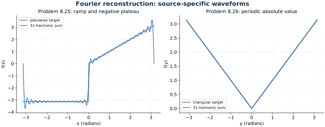
Fourier partial sums reconstruct the ramp/step waveform and the triangular waveform from their independently calculated coefficients.
Problem 8.22 — prove equivalence of amplitude-phase and sine-cosine Fourier forms
Paraphrased task. Prove equivalence of amplitude-phase and sine-cosine fourier forms.
Formula reference. Use (1), its definitions, and the topic illustration.
Worked application.
Set the fundamental spatial frequency \(k_0=2\pi/L\). Expand each phase-shifted term using \(\cos(mk_0x+\epsilon_m)=\cos\epsilon_m\cos(mk_0x)-\sin\epsilon_m\sin(mk_0x)\).
Identify the sine-cosine coefficients as \(a_m=C_m\cos\epsilon_m\), \(b_m=-C_m\sin\epsilon_m\), and the constant as \(C_0=a_0/2\).
Conversely, take \(C_m=\sqrt{a_m^2+b_m^2}\) and \(\epsilon_m=\operatorname{atan2}(-b_m,a_m)\). The two-argument angle keeps the correct quadrant; when \(C_m=0\), that harmonic’s phase is arbitrary.
Result. The amplitude-phase and sine-cosine forms are equivalent term by term.
Check. The minus sign in \(b_m=-C_m\sin\epsilon_m\) comes from the plus sign inside \(\cos(mk_0x+\epsilon_m)\).
Problem 8.23 — show screw symmetry removes even harmonics
Paraphrased task. Show screw symmetry removes even harmonics.
Formula reference. Use (1), its definitions, and the topic illustration.
Worked application.
Suppose \(f(x+L/2)=-f(x)\). Split a complex Fourier coefficient into two half-period integrals:
\[c_m=\frac1L\left[\int_0^{L/2}f(x)e^{-imk_0x}\,dx +\int_{L/2}^{L}f(x)e^{-imk_0x}\,dx\right].\]In the second integral substitute \(x=u+L/2\). Its integrand becomes \(-f(u)e^{-imk_0u}e^{-im\pi}=-(-1)^mf(u)e^{-imk_0u}\).
Thus \(c_m=[1-(-1)^m]L^{-1}\int_0^{L/2}f(u)e^{-imk_0u}\,du\). Every even coefficient, including DC, vanishes; only odd harmonics can remain.
Result. Half-wave antisymmetry removes the DC term and all even harmonics.
Check. Odd harmonics can contain both sine and cosine terms unless an additional odd/even spatial parity is specified.
Problem 8.24 — state when only even harmonics remain
Paraphrased task. State when only even harmonics remain.
Formula reference. Use (1), its definitions, and the topic illustration.
Worked application.
Suppose the function repeats after \(L/2\), even though its Fourier series is expressed on an interval of length \(L\).
Split the coefficient integral into two halves as in Problem 8.23. Now \(f(u+L/2)=f(u)\), so the multiplier is \(1+(-1)^m\).
This vanishes for every odd \(m\), leaving only even harmonics relative to \(k_0=2\pi/L\), plus possible DC. Relative to the true shorter period, these are simply ordinary integer harmonics.
Result. Only even harmonics relative to period \(L\) remain when the function also has period \(L/2\).
Check. Harmonic parity depends on the chosen reference period; it is not an intrinsic label independent of that choice.
Problem 8.25 — derive the series of a periodic ramp-and-step waveform
Paraphrased task. Derive the series of a periodic ramp-and-step waveform.
Formula reference. Use (1), its definitions, and the topic illustration.
Worked application.
Read one period of the source graph as \(f(x)=-\pi\) for \(-\pi<x<0\) and \(f(x)=x\) for \(0<x<\pi\), extended with period \(2\pi\). Its mean is \([-\pi^2+\pi^2/2]/(2\pi)=-\pi/4\).
Split the coefficient integrals at zero. The cosine integral gives \(a_m=[(-1)^m-1]/(\pi m^2)\). For sine, the constant segment contributes \([1-(-1)^m]/m\), while integration by parts of \(x\sin mx\) contributes \(-(-1)^m/m\).
Therefore
\[f(x)=-\frac\pi4-\frac2\pi\sum_{j=0}^{\infty} \frac{\cos[(2j+1)x]}{(2j+1)^2} +\sum_{m=1}^{\infty}\frac{1-2(-1)^m}{m}\sin(mx).\]The first sine terms are \(3\sin x-\tfrac12\sin2x+\sin3x-\tfrac14\sin4x\).
Result. The series contains odd cosines and both odd and even sines; the waveform is neither even nor odd.
Check. At \(x=0\) the series converges to the jump midpoint \(-\pi/2\), not to either one-sided value.
Problem 8.26 — derive the series of a second periodic waveform
Paraphrased task. Derive the series of a second periodic waveform.
Formula reference. Use (1), its definitions, and the topic illustration.
Worked application.
The triangular graph is \(f(y)=|y|\) on \([-\pi,\pi]\), extended periodically. It is even, so \(b_m=0\).
The mean is \(a_0/2=(1/\pi)\int_0^\pi y\,dy=\pi/2\). Integration by parts gives \(a_m=(2/\pi)\int_0^\pi y\cos(my)\,dy=2[(-1)^m-1]/(\pi m^2)\).
Even coefficients vanish; odd coefficients are \(-4/(\pi m^2)\). Hence \(f(y)=\pi/2-(4/\pi)\sum_{j=0}^{\infty}\cos[(2j+1)y]/(2j+1)^2\).
Result. \(f(y)=\pi/2-(4/\pi)(\cos y+\cos3y/9+\cos5y/25+\cdots)\).
Check. At \(y=0\), \(\sum_{j\ge0}(2j+1)^{-2}=\pi^2/8\) makes the reconstructed value zero.
Problem 8.27 — generalize the waveform to arbitrary period
Paraphrased task. Generalize the waveform to arbitrary period.
Formula reference. Use (1), its definitions, and the topic illustration.
Worked application.
The generalized triangle has period \(L\), minimum zero at \(y=0\), and maximum \(H\) at \(y=\pm L/2\). On the centred period it is \(f(y)=2H|y|/L\).
Scale the previous solution’s coordinate by \(u=2\pi y/L\) and amplitude by \(H/\pi\), so \(f(y)=(H/\pi)|u|\) on that period.
The scaled series is
\[f(y)=\frac H2-\frac{4H}{\pi^2} \sum_{j=0}^{\infty} \frac{\cos[2\pi(2j+1)y/L]}{(2j+1)^2}.\]
Result. The mean is \(H/2\); odd cosine amplitudes scale as \(-4H/[\pi^2(2j+1)^2]\).
Check. Setting \(H=\pi\) and \(L=2\pi\) recovers Problem 8.26 exactly.
Problem 8.28 — obtain a shifted series by changing axes
Paraphrased task. Obtain a shifted series by changing axes.
Formula reference. Use (1), its definitions, and the topic illustration.
Worked application.
The shifted graph has a peak \(\pi/2\) at zero and troughs \(-\pi/2\) at \(\pm\pi\). On the centred period it is \(g(y)=\pi/2-|y|\).
Subtract the entire series from Problem 8.26 from \(\pi/2\). The constant term cancels and every nonzero coefficient changes sign.
Thus \(g(y)=(4/\pi)\sum_{j=0}^{\infty}\cos[(2j+1)y]/(2j+1)^2\). Equivalently, a half-period shift of the zero-mean triangle reverses the signs of all its odd harmonics.
Result. \(g(y)=(4/\pi)(\cos y+\cos3y/9+\cos5y/25+\cdots)\).
Check. The absence of a DC term matches the equal positive and negative areas of this centred triangular waveform.
Problem 8.29 — derive the series of a full-wave rectified sine
Paraphrased task. Derive the series of a full-wave rectified sine.
Formula reference. Use (1), its definitions, and the topic illustration.
Worked application.
A full-wave rectified sinusoid with a 1 s period is \(f(t)=E_0|\sin\pi t|\), whose unrectified parent has a 2 s period.
Over \(0<t<1\), \(f=E_0\sin\pi t\). The mean is \(\int_0^1f\,dt=2E_0/\pi\). Product-to-sum integration gives \(a_m=2E_0\int_0^1\sin\pi t\cos2\pi mt\,dt=-4E_0/[\pi(4m^2-1)]\); sine coefficients vanish by symmetry.
Therefore
\[f(t)=\frac{2E_0}\pi-\frac{4E_0}\pi \sum_{m=1}^{\infty}\frac{\cos(2\pi mt)}{4m^2-1}.\]
Result. The first cosine denominators are \(3,15,35,\ldots\), with a 1 Hz fundamental after rectification.
Check. Using \(|\sin2\pi t|\) would instead give a 0.5 s rectified period.
Fourier transforms
Formula and definitions.
Insert the piecewise support before integrating. Modulation shifts spectra: \(\mathcal F\{f(x)e^{ik_0x}\}=F(k-k_0)\), while multiplication by \(x\) gives \(i\,dF/dk\). Complete the square for a Gaussian and use the delta sifting property for constants and impulses.
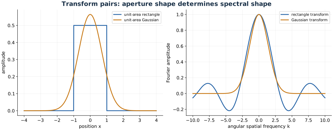
A rectangular window transforms to a sinc; a Gaussian transforms to a Gaussian without the ideal sinc’s sidelobes.
Problem 8.30 — transform a square pulse with complex exponentials
Paraphrased task. Transform a square pulse with complex exponentials.
Formula reference. Use (2), its definitions, and the topic illustration.
Worked application.
These notes use \(F(k)=\int f(x)e^{-ikx}\,dx\), whereas the source uses the opposite exponential sign in some endpoints. Let the pulse be \(E_0\) on \([-L,L]\) and zero elsewhere.
Direct integration gives \(F(k)=E_0[e^{-ikx}/(-ik)]_{-L}^{L}=E_0(e^{ikL}-e^{-ikL})/(ik)\).
Euler’s identity reduces this to \(F(k)=2E_0\sin(kL)/k=2E_0L\operatorname{sinc}(kL)\), where \(\operatorname{sinc}u=\sin u/u\). At zero frequency use the continuous limit.
Result. \(F(k)=2E_0L\operatorname{sinc}(kL)\).
Check. \(F(0)=2LE_0\) equals the pulse area; the even real pulse must have an even real transform under either sign convention.
Problem 8.31 — transform a windowed sine wave
Paraphrased task. Transform a windowed sine wave.
Formula reference. Use (2), its definitions, and the topic illustration.
Worked application.
Write the windowed sine as \(f(x)=E_0P_L(x)[e^{ik_px}-e^{-ik_px}]/(2i)\), where \(P_L=1\) for \(|x|\le L\).
The rectangular-window transform is \(W(k)=2L\operatorname{sinc}(kL)\). Modulation shifts it: \(\mathcal F\{P_Le^{\pm ik_px}\}=W(k\mp k_p)\).
Consequently
\[F(k)=\frac{E_0L}{i} \left\{\operatorname{sinc}[(k-k_p)L] -\operatorname{sinc}[(k+k_p)L]\right\}.\]The source’s \(+ikx\) forward convention reverses this imaginary transform’s sign.
Result. The spectrum is the imaginary, antisymmetric difference of two shifted sinc lobes.
Check. The input is real and odd, so \(F(-k)=-F(k)=F(k)^*\) and \(F(0)=0\).
Problem 8.32 — transform a windowed sine-squared wave
Paraphrased task. Transform a windowed sine-squared wave.
Formula reference. Use (2), its definitions, and the topic illustration.
Worked application.
Apply \(\sin^2k_px=(1-\cos2k_px)/2\) within the same \([-L,L]\) window.
The constant-window term transforms to \(E_0L\operatorname{sinc}(kL)\). The cosine term is the sum of two exponentials, each shifted by \(\pm2k_p\) and weighted by \(-E_0/4\) before multiplying the window transform.
Thus
\[F(k)=E_0L\left\{\operatorname{sinc}(kL) -\frac12\operatorname{sinc}[(k-2k_p)L] -\frac12\operatorname{sinc}[(k+2k_p)L]\right\}.\]
Result. A central sinc lobe minus two half-weight sinc lobes centred at \(\pm2k_p\).
Check. \(F(0)=E_0[L-\sin(2k_pL)/(2k_p)]\), equal to the integral of the windowed sine squared.
Problem 8.33 — transform a two-sided exponential by two routes
Paraphrased task. Transform a two-sided exponential by two routes.
Formula reference. Use (2), its definitions, and the topic illustration.
Worked application.
The plotted function is the two-sided even exponential \(f(x)=e^{-a|x|}\), with \(a>0\), not a one-sided exponential. Parity removes the sine contribution.
Directly, \(F(k)=2\int_0^\infty e^{-ax}\cos(kx)\,dx=2\operatorname{Re}[1/(a+ik)]=2a/(a^2+k^2)\).
Alternatively, split \(f=H(x)e^{-ax}+H(-x)e^{ax}\). The two transforms are \(1/(a+ik)\) and \(1/(a-ik)\); adding them gives the same Lorentzian.
Result. \(F(k)=2a/(a^2+k^2)\).
Check. \(F(0)=2/a\) matches the total area, and the result is even and real.
Problem 8.34 — transform a Gaussian and interpret apodization
Paraphrased task. Transform a gaussian and interpret apodization.
Formula reference. Use (2), its definitions, and the topic illustration.
Worked application.
Let \(f(x)=\sqrt{a/\pi}\,e^{-ax^2}\), \(a>0\). In the transform exponent, complete the square: \(-ax^2-ikx=-a(x+ik/(2a))^2-k^2/(4a)\).
The Gaussian integral contributes \(\sqrt{\pi/a}\), cancelling the normalization. Equivalently, integration by parts gives \(F'(k)=-kF(k)/(2a)\) with \(F(0)=1\). Both routes yield \(F(k)=e^{-k^2/(4a)}\).
A smoothly Gaussian pupil amplitude has a Gaussian Fourier field with no sidelobes in the ideal untruncated model. Gaussian apodization suppresses Airy rings at the cost of throughput and a broader central image; a finite hard truncation can leave residual rings.
Result. \(\mathcal F\{\sqrt{a/\pi}e^{-ax^2}\}=e^{-k^2/(4a)}\).
Check. Making the spatial Gaussian narrower by increasing \(a\) broadens its Fourier transform, as expected from reciprocal width scaling.
Problem 8.35 — transform a causal exponentially weighted coordinate
Paraphrased task. Transform a causal exponentially weighted coordinate.
Formula reference. Use (2), its definitions, and the topic illustration.
Worked application.
The step function restricts support to \(x\ge0\), so \(F(k)=\int_0^\infty xe^{-(a+ik)x}\,dx\), with \(a>0\) ensuring convergence.
Start from \(\int_0^\infty e^{-(a+ik)x}\,dx=1/(a+ik)\). Differentiate with respect to \(a\) and change sign to insert the factor \(x\).
This gives \(F(k)=-\partial_a[1/(a+ik)]=1/(a+ik)^2\). Under a \(+ikx\) forward-transform convention, it becomes the source’s \(1/(a-ik)^2\).
Result. \(F(k)=1/(a+ik)^2\) with the negative-exponential convention used here.
Check. \(F(0)=1/a^2=\int_0^\infty xe^{-ax}\,dx\), and \(F(-k)=F(k)^*\).
Problem 8.36 — transform delta and constant functions
Paraphrased task. Transform delta and constant functions.
Formula reference. Use (2), its definitions, and the topic illustration.
Worked application.
Apply delta sifting: \(\mathcal F\{\delta(x)\}=\int\delta(x)e^{-ikx}\,dx=e^0=1\).
The inverse transform of a frequency delta is \((2\pi)^{-1}\int2\pi\delta(k)e^{ikx}\,dk=1\).
Therefore \(\mathcal F\{1\}=2\pi\delta(k)\). The second relation is a distribution identity, not an ordinary convergent integral of a constant over the whole real line.
Result. \(\delta(x)\leftrightarrow1\) and \(1\leftrightarrow2\pi\delta(k)\).
Check. The factor \(2\pi\) is fixed by the chosen inverse-transform normalization.
Convolution
Formula and definitions.
For a graphical convolution, reverse one function, translate it by \(x\), multiply overlaps, and integrate. For impulses, form every ordered pair of locations; their coordinates add and coincident sums add weights. The transform product/convolution theorem follows by inserting the inverse transforms and evaluating the inner exponential integral as a delta.
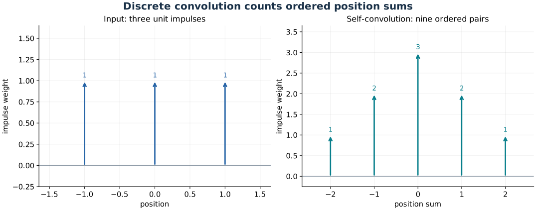
Convolution adds positions and multiplies weights. Three unit impulses produce the five-weight sequence 1, 2, 3, 2, 1.
Problem 8.37 — prove the frequency-domain convolution theorem
Paraphrased task. Prove the frequency-domain convolution theorem.
Formula reference. Use (3), its definitions, and the topic illustration.
Worked application.
Insert the inverse transform of \(h\): \(h(x)=(2\pi)^{-1}\int H(q)e^{iqx}\,dq\) into \(\mathcal F\{fh\}=\int f(x)h(x)e^{-ikx}\,dx\).
Interchange the integrals when they are absolutely integrable, or interpret the result distributionally where appropriate. The inner integral is \(\int f(x)e^{-i(k-q)x}\,dx=F(k-q)\).
Hence
\[\mathcal F\{f h\}(k)=\frac1{2\pi}\int H(q)F(k-q)\,dq =\frac1{2\pi}(F*H)(k).\]
Result. Multiplication in position corresponds to frequency convolution divided by \(2\pi\).
Check. The dual theorem \(\mathcal F\{f*h\}=FH\) has no extra factor in this convention.
Problem 8.38 — transform a cosine squared using spectral convolution
Paraphrased task. Transform a cosine squared using spectral convolution.
Formula reference. Use (3), its definitions, and the topic illustration.
Worked application.
The cosine spectrum is \(F(k)=\pi[\delta(k-k_0)+\delta(k+k_0)]\).
Self-convolution produces four ordered pairs: the equal-sign pairs land at \(\pm2k_0\), while the two opposite-sign pairs coincide at zero. Thus \(F*F=\pi^2[\delta(k-2k_0)+2\delta(k)+\delta(k+2k_0)]\).
Multiply by \(1/(2\pi)\) from the product theorem:
\[\mathcal F\{\cos^2k_0x\} =\pi\delta(k)+\frac\pi2[\delta(k-2k_0)+\delta(k+2k_0)].\]
Result. Three spectral lines: DC weight \(\pi\), and weights \(\pi/2\) at \(\pm2k_0\).
Check. Directly transforming \(\cos^2k_0x=(1+\cos2k_0x)/2\) gives the same weights.
Problem 8.39 — prove commutativity of convolution
Paraphrased task. Prove commutativity of convolution.
Formula reference. Use (3), its definitions, and the topic illustration.
Worked application.
Begin with \((f*h)(x)=\int_{-\infty}^{\infty}f(\xi)h(x-\xi)\,d\xi\).
Substitute \(u=x-\xi\), so \(d\xi=-du\). The lower and upper integration limits exchange; the Jacobian minus sign restores their usual order.
The result is \(\int_{-\infty}^{\infty}h(u)f(x-u)\,du=(h*f)(x)\). Thus either function can be the one reflected and translated in the graphical construction.
Result. \(f*h=h*f\) whenever the convolution is well defined.
Check. Convolution is commutative, whereas correlation generally changes by reversal or conjugation when its arguments are exchanged.
Problem 8.40 — construct a discrete self-convolution
Paraphrased task. Construct a discrete self-convolution.
Formula reference. Use (3), its definitions, and the topic illustration.
Worked application.
The graph contains three unit impulses at \(-1,0,1\), so \(f(x)=\delta(x+1)+\delta(x)+\delta(x-1)\).
Form all nine ordered sums of positions. The sum \(-2\) occurs once, \(-1\) twice, zero three times, \(1\) twice, and \(2\) once.
Draw impulses at those five positions with weights \(1,2,3,2,1\); these are weights (areas), not finite impulse heights. Algebraically the result is \(\delta(x+2)+2\delta(x+1)+3\delta(x)+2\delta(x-1)+\delta(x-2)\).
Result. The self-convolution is the five-line triangular weight sequence \(1,2,3,2,1\).
Check. The output total weight is \(9=3^2\), the product of the two input total weights.
Problem 8.41 — convolve a three-impulse distribution with itself
Paraphrased task. Convolve a three-impulse distribution with itself.
Formula reference. Use (3), its definitions, and the topic illustration.
Worked application.
Use the delta identity directly: \(\int\delta(\xi-a)\delta(x-\xi-b)\,d\xi=\delta[x-(a+b)]\).
Expand the product of the three terms in \(f=\delta(x-1)+\delta(x)+\delta(x+1)\) with another copy of \(f\). Keep all ordered pairs, including the two ways to form each nonzero inner sum and the three ways to form zero.
Collect coincident deltas:
\[(f*f)(x)=\delta(x-2)+2\delta(x-1)+3\delta(x) +2\delta(x+1)+\delta(x+2).\]
Result. The analytic expansion confirms the graphical construction in Problem 8.40.
Check. Replacing ordered pairs with only distinct unordered pairs would undercount the cross terms.
Problem 8.42 — self-convolve a four-line spectrum
Paraphrased task. Self-convolve a four-line spectrum.
Formula reference. Use (3), its definitions, and the topic illustration.
Worked application.
The four unit spectral impulses lie at \(-3,-2,2,3\). Write \(F(k)=\sum_{a\in\{-3,-2,2,3\}}\delta(k-a)\).
Sum every ordered pair. The outer equal pairs give weights one at \(\pm6,\pm4\); mixed same-sign pairs give weight two at \(\pm5\); mixed opposite-sign pairs give weight two at \(\pm1\); the four exactly opposite pairs give weight four at zero.
Consequently
\[F*F=4\delta(k)+2[\delta(k-1)+\delta(k+1)+\delta(k-5)+\delta(k+5)] +\delta(k-4)+\delta(k+4)+\delta(k-6)+\delta(k+6).\]
Result. Nine output locations \(-6,-5,-4,-1,0,1,4,5,6\) with weights \(1,2,1,2,4,2,1,2,1\).
Check. The weights sum to \(16=4^2\); there are no lines at \(\pm2\) or \(\pm3\).
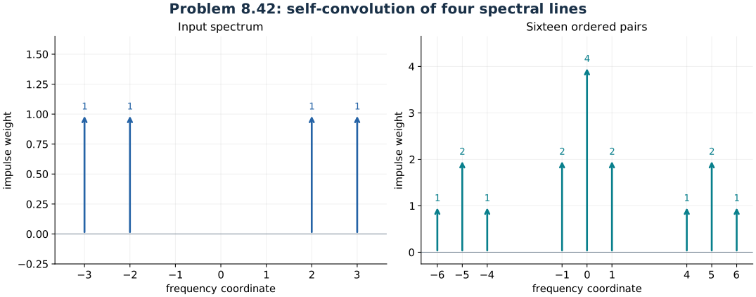
All sixteen ordered sums of four spectral positions give nine distinct output positions with the displayed multiplicities.
Problem 8.43 — convolve a rectangular pulse with an impulse pair and transform it
Paraphrased task. Convolve a rectangular pulse with an impulse pair and transform it.
Formula reference. Use (3), its definitions, and the topic illustration.
Worked application.
Let \(p(x)=E_0\) on \([-d/2,d/2]\) and zero outside. The impulse pair is signed: \(h(x)=\delta(x-d/2)-\delta(x+d/2)\).
Sifting gives \(g(x)=p(x-d/2)-p(x+d/2)\): it is \(-E_0\) on \((-d,0)\), \(+E_0\) on \((0,d)\), and zero elsewhere.
The transforms are \(P(k)=E_0d\operatorname{sinc}(kd/2)\) and \(H(k)=-2i\sin(kd/2)\). Multiply them:
\[G(k)=-2iE_0d\operatorname{sinc}(kd/2)\sin(kd/2).\]
Result. The convolution is an odd bipolar rectangular pulse; its transform is the imaginary product of a sinc envelope and a sine.
Check. The opposite-sign lobes have zero total area, so \(G(0)=0\).
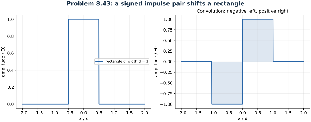
A rectangle convolved with an opposite-sign impulse pair becomes a bipolar rectangle with zero total area.
Problem 8.44 — self-convolve a double-slit aperture function
Paraphrased task. Self-convolve a double-slit aperture function.
Formula reference. Use (3), its definitions, and the topic illustration.
Worked application.
Let each unit-height slit have width \(b\), with centre separation \(d\). Write \(f(x)=p_b(x-d/2)+p_b(x+d/2)\).
A rectangle convolved with itself is its overlap length: \(T_b(x)=(b-|x|)_+\), where \((u)_+=\max(u,0)\).
Expand the four shifted pairings. The two same-side pairings are centred at \(\pm d\), while the two cross pairings coincide at zero:
\[(f*f)(x)=T_b(x-d)+2T_b(x)+T_b(x+d).\]
Result. Three triangular components of base width \(2b\), with central peak twice either outer peak when they do not overlap.
Check. Their total area is \(4b^2=(2b)^2\), as required by the convolution area rule.
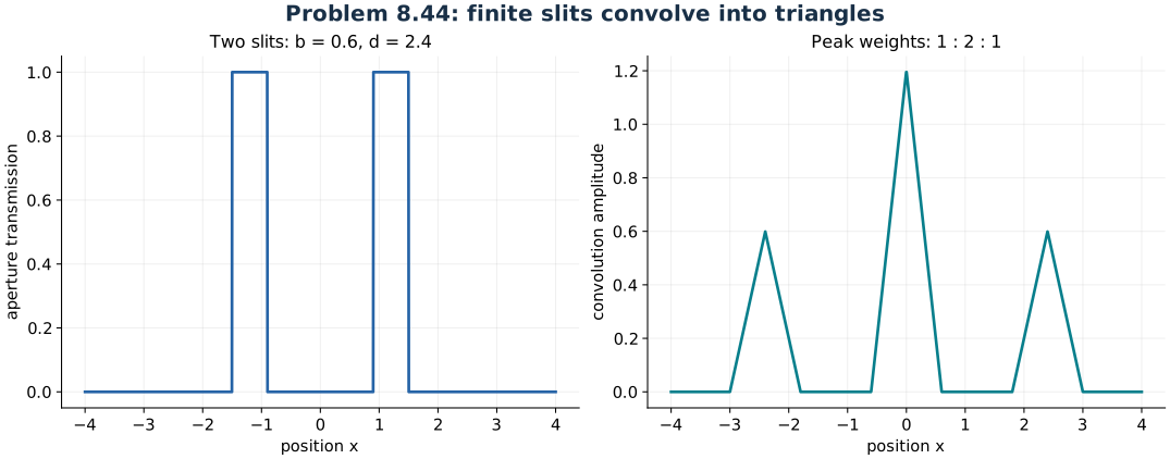
Self-convolution of two finite slits creates three triangular components, including two coincident cross terms at the centre.
Problem 8.45 — convolve two unequal rectangular pulses
Paraphrased task. Convolve two unequal rectangular pulses.
Formula reference. Use (3), its definitions, and the topic illustration.
Worked application.
The actual source graph shows two finite rectangles: height \(A\) on \([1,2]\) and height \(B\) on \([3,5]\). The tick marks depict \(A=2\), \(B=1\); keeping \(A,B\) symbolic makes the normalization explicit.
In the convolution integral the allowed overlap is \([1,2]\cap[x-5,x-3]\). Its length is \(\max[0,\min(2,x-3)-\max(1,x-5)]\).
Hence the output is zero outside \([4,7]\), rises as \(AB(x-4)\) on \([4,5]\), stays at \(AB\) on \([5,6]\), and falls as \(AB(7-x)\) on \([6,7]\). The resulting trapezoid has height 2 for the illustrated normalization.
Result. A trapezoid supported on \([4,7]\), with a flat top on \([5,6]\) and peak \(AB\).
Check. Its area is \(2AB=(A\cdot1)(B\cdot2)\), matching the product of rectangle areas.
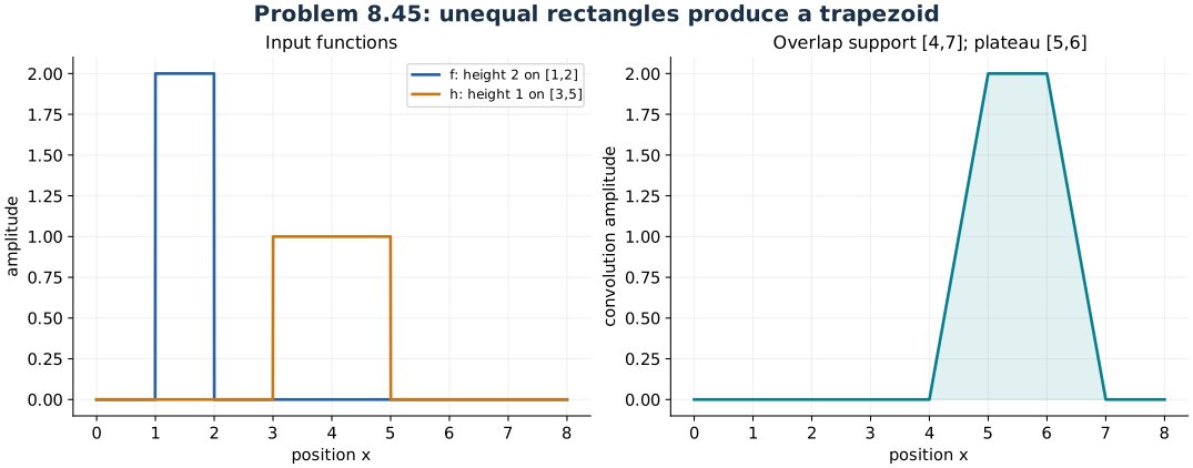
The overlap length of unequal rectangles grows, plateaus, then decreases, producing a trapezoid rather than a triangle.
Problem 8.46 — construct a further graphical convolution
Paraphrased task. Construct a further graphical convolution.
Formula reference. Use (3), its definitions, and the topic illustration.
Worked application.
The input impulses at \(x=0,1,2,3,4,5\) have respective weights \(1,2,3,1,1,2\). The spread function is the unit triangle \(h(x)=(1-|x|)_+\).
Delta sifting turns the convolution into shifted weighted copies:
\[g(x)=h(x)+2h(x-1)+3h(x-2)+h(x-3)+h(x-4)+2h(x-5).\]Each triangle is zero at neighbouring integer centres, so \(g\) passes through \((-1,0),(0,1),(1,2),(2,3),(3,1),(4,1),(5,2),(6,0)\). Join consecutive points by straight segments and set the curve to zero outside \([-1,6]\).
Result. The result is the piecewise-linear interpolation of the six impulse weights, with zero endpoints at \(-1\) and \(6\).
Check. The triangle area is one, so the output area equals the input weight sum \(10\).
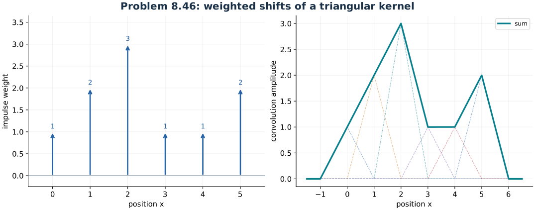
Shifted weighted triangular kernels add to the piecewise-linear interpolation of the impulse weights.
Problem 8.47 — self-convolve a two-dimensional six-hole mask
Paraphrased task. Self-convolve a two-dimensional six-hole mask.
Formula reference. Use (3), its definitions, and the topic illustration.
Worked application.
Let the six hole centres be the vertices \(\mathbf r_j\) of a regular hexagon of circumradius \(a\), and let \(p(\mathbf r)\) denote one circular hole. Then \(f=\sum_jp(\mathbf r-\mathbf r_j)\) and \(f*f=\sum_{j,l}(p*p)(\mathbf r-\mathbf r_j-\mathbf r_l)\).
The 36 ordered centre sums form 19 distinct positions: one central position of multiplicity 6, six positions at radius \(a\) of multiplicity 2, six at radius \(\sqrt3a\) of multiplicity 2, and six at radius \(2a\) of multiplicity 1. The middle-radius hexagon is rotated \(30^\circ\) relative to the others.
Finite holes do not convolve to uniform disks. If each hole has radius \(r_0\), the individual spot profile is the disk-overlap area
\[(p*p)(\rho)=2r_0^2\arccos\frac{\rho}{2r_0} -\frac{\rho}{2}\sqrt{4r_0^2-\rho^2},\quad 0\le\rho\le2r_0,\]and zero beyond \(2r_0\). Place copies of this profile at the 19 centres with the stated multiplicities, adding overlaps if necessary.
Result. Nineteen hexagonally arranged convolution spots, with multiplicities \(6\) at the centre, \(2\) on each of two inner rings, and \(1\) on the outer ring.
Check. The multiplicities total \(6+6(2)+6(2)+6(1)=36\), accounting for every ordered pair of the six holes.
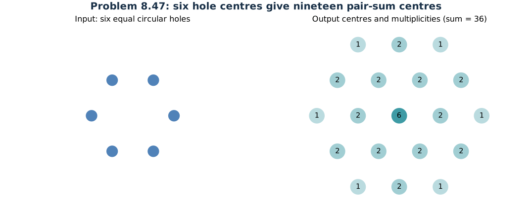
The six-hole mask has nineteen distinct pair-sum centres. Labels give convolution multiplicities, not physical hole diameters.