Chapter 1: Wave Motion
Source: Eugene Hecht, Schaum’s Outline of Theory and Problems of Optics (1975), Chapter 1. The entries below cover only the chapter’s Supplementary Problems; prompts are paraphrased and are not reproduced.
Each numbered solution states its assumptions, develops the algebra, substitutes the relevant data, and checks the result. Original SVG illustrations show the ray geometry, field relationships, or calculated curves. Diagrams are schematic unless their axes specify a scale. Source inconsistencies and approximations are identified explicitly rather than silently copied into the answer.
The wave equation
Formula and definitions.
Put \(u=x\mp vt\). The chain rule gives \(y_x=f'(u)\), \(y_{xx}=f''(u)\), \(y_t=\mp vf'(u)\), and \(y_{tt}=v^2f''(u)\). Substitution proves the differential equation. A plus sign in \(x+vt\) moves a fixed value of \(u\) toward decreasing \(x\); a minus sign moves it toward increasing \(x\).
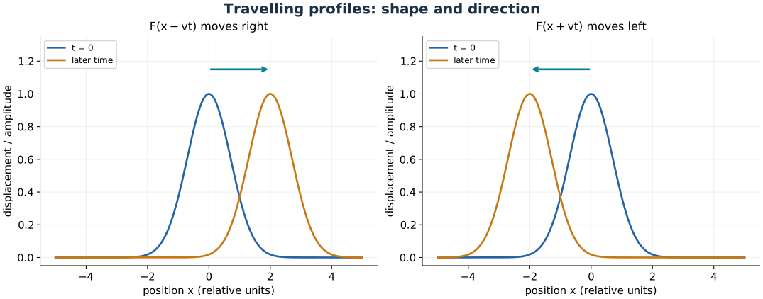
A translated pulse keeps its shape: positive and negative phase signs select opposite propagation directions.
Problem 1.31 — test a squared-sine travelling profile
Paraphrased task. Test a squared-sine travelling profile.
Formula reference. Use (1), its definitions, and the topic illustration.
Worked application.
The printed argument is \(u=4\pi(t+z)\). Differentiate the squared sine before differentiating its argument: \(d(\sin^2u)/du=\sin2u\).
The first derivatives are \(\psi_t=4\pi A\sin2u\) and \(\psi_z=4\pi A\sin2u\); differentiating again gives
\[\psi_{tt}=32\pi^2A\cos2u,\qquad \psi_{zz}=32\pi^2A\cos2u.\]Therefore \(\psi_{zz}=\psi_{tt}/v^2\) with \(v=1\) in the stated coordinate units. A fixed value of \(t+z\) has \(dz/dt=-1\).
Result. The profile satisfies the wave equation and translates toward negative \(z\) at unit speed.
Check. The factor of two from differentiating \(\sin2u\) appears in both second derivatives; the speed follows their ratio, not the sine’s period.
Problem 1.32 — distinguish progressive from non-progressive functions
Paraphrased task. Distinguish progressive from non-progressive functions.
Formula reference. Use (1), its definitions, and the topic illustration.
Worked application.
For \(\psi_1=A(x-t)^2\), put \(u=x-t\); it is a fixed profile translating at \(+1\).
The affine expression \(\psi_2=A(y+t+B)\) is also \(F(y+t)\). Its second derivatives both vanish, so the differential equation cannot determine a unique speed; tracking a fixed level gives velocity \(-1\).
For the quadratic-phase sine, set \(u=B(x^2-Ct^2)\). The first-derivative ratio is
\[-\frac{\psi_t}{\psi_x}=\frac{Ct}{x}.\]This is not a constant translation speed. For \(\psi_4=A/(Bx^2-t)\), the same ratio is \(1/(2Bx)\), again position dependent. Singular points are excluded.
Result. For generic nonzero constants, the nondegenerate travelling wave is \(\psi_1\); \(\psi_2\) is a degenerate affine travelling profile. The printed answer lists only \(\psi_1\).
Check. A rigidly translated differentiable profile obeys \(\psi_t=-v\psi_x\) with constant \(v\); satisfying a second-order equation trivially is a separate issue.
Problem 1.33 — recover speed and direction from three profiles
Paraphrased task. Recover speed and direction from three profiles.
Formula reference. Use (1), its definitions, and the topic illustration.
Worked application.
Write the first argument as \(y-t\); its constant-level trajectory is \(y=t+u_0\).
Factor the second argument as \(B[x+(C/B)t+D/B]\). Its velocity is \(dx/dt=-C/B\).
Complete the square in the exponential:
\[Bz^2+BC^2t^2-2BCzt=B(z-Ct)^2.\]Thus its constant profile moves with \(dz/dt=C\). Speeds are absolute values; directions quoted below assume positive \(B,C\).
Result. The velocities are \(+1\,\hat{\mathbf y}\), \(-(C/B)\hat{\mathbf x}\), and \(C\hat{\mathbf z}\).
Check. The offset \(D\) changes the origin of the profile but cannot change its velocity.
Problem 1.34 — prove that an arbitrary profile moving toward negative x is progressive
Paraphrased task. Prove that an arbitrary profile moving toward negative x is progressive.
Formula reference. Use (1), its definitions, and the topic illustration.
Worked application.
At \(t=0\), denote the graph by \(G(x)=g(x)\). At a later time the value at \(x\) is \(G(x+vt)\).
Follow a recognizable point initially at \(x_0\). It remains the same point when \(x+vt=x_0\), so \(x=x_0-vt\).
Any two such points have separation \(x_b(t)-x_a(t)=x_{b0}-x_{a0}\). Their heights and separation remain unchanged, establishing translation without distortion.
Result. \(g(x+vt)\) is a rigid profile travelling toward \(-x\) for \(v>0\).
Check. Replacing \(t\) by \(t+\Delta t\) shifts every feature left by \(v\Delta t\), as shown in the wave-profile diagram.
Problem 1.35 — test a superposition of oppositely travelling profiles
Paraphrased task. Test a superposition of oppositely travelling profiles.
Formula reference. Use (1), its definitions, and the topic illustration.
Worked application.
Complete the square \(Cx^2+B^2Ct^2-2BCxt=C(x-Bt)^2\).
Define \(G(u)=A(u+D)^2\) and \(F(u)=Ae^{Cu^2}\). The disturbance is \(G(x+Bt)+F(x-Bt)\).
Differentiate each term using its own travelling coordinate:
\[\psi_{xx}=G''+F'',\qquad \psi_{tt}=B^2G''+B^2F''=B^2\psi_{xx}.\]Linearity permits adding the two solutions, even though they move in opposite directions.
Result. The sum solves the wave equation with speed magnitude \(|B|\); it is generally not one rigidly translating profile.
Check. The two components must have the same speed magnitude for their sum to satisfy this one wave equation.
Problem 1.36 — verify an arbitrary twice-differentiable travelling profile
Paraphrased task. Verify an arbitrary twice-differentiable travelling profile.
Formula reference. Use (1), its definitions, and the topic illustration.
Worked application.
Set \(u=t-x/v\), with constant nonzero \(v\) and a twice-differentiable function \(h\).
Apply the chain rule twice:
\[\psi_t=h'(u),\quad \psi_{tt}=h''(u),\quad \psi_x=-h'(u)/v,\quad \psi_{xx}=h''(u)/v^2.\]Subtract the two sides of the wave equation; the remainder is identically zero. Following \(u=u_0\) gives \(x=v(t-u_0)\).
Result. \(h(t-x/v)\) is a wave travelling at signed velocity \(v\).
Check. The minus sign in the first spatial derivative disappears after the second derivative.
Problem 1.37 — relate the temporal and spatial rates of change
Paraphrased task. Relate the temporal and spatial rates of change.
Formula reference. Use (1), its definitions, and the topic illustration.
Worked application.
For a right-travelling profile \(\psi=F(x-vt)\), differentiate while holding the other independent variable fixed.
The resulting relations \(\psi_x=F'\) and \(\psi_t=-vF'\) eliminate the unknown profile derivative:
\[\psi_t=-v\psi_x.\]For \(G(x+vt)\) the sign is positive. A sum of right- and left-travelling waves generally does not satisfy either first-order relation with one sign.
Result. The multiplicative constant is \(-v\) for rightward motion and \(+v\) for leftward motion.
Check. The units are displacement/time on both sides because \(v\psi_x\) supplies the missing length/time factor.
Sinusoidal waves
Formula and definitions.
A repetition in time requires \(\omega T=2\pi m\); the fundamental period uses \(m=1\). Likewise a spatial repetition requires \(k\lambda=2\pi\). Holding the phase constant yields \(dx/dt=\pm\omega/k\), which fixes the propagation direction.
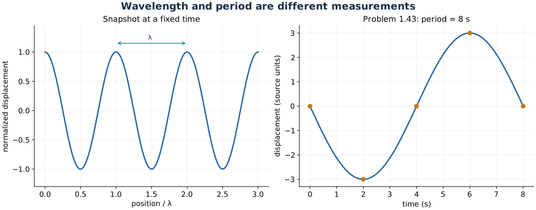
Spatial and temporal sections of a sinusoid distinguish wavelength from period; the time trace uses Problem 1.43.
Problem 1.38 — derive temporal periodicity of a harmonic wave
Paraphrased task. Derive temporal periodicity of a harmonic wave.
Formula reference. Use (2), its definitions, and the topic illustration.
Worked application.
At fixed position, advancing the time by \(T\) changes the phase of \(A\sin(kx-\omega t+\phi)\) by \(-\omega T\).
To repeat the entire waveform, rather than just one accidental value of the sine, this change must be \(2\pi\) times an integer.
The smallest positive repeat uses \(\omega T=2\pi\), hence \(T=2\pi/\omega\). Combining \(\omega=2\pi f\) and \(v=f\lambda\) also gives \(T=\lambda/v\).
Result. \(T=2\pi/\omega=1/f=\lambda/v\).
Check. A half-period changes the sign of a sine; it does not reproduce a general instantaneous displacement.
Problem 1.39 — convert radio frequency to wavelength and back
Paraphrased task. Convert radio frequency to wavelength and back.
Formula reference. Use (2), its definitions, and the topic illustration.
Worked application.
Electromagnetic waves in vacuum have \(v=c\simeq3.00\times10^8\,\mathrm{m/s}\).
At \(f=100\,\mathrm{Hz}\), use \(\lambda=c/f=(3.00\times10^8)/100=3.00\times10^6\,\mathrm m\).
For a one-metre wavelength, reverse the calculation: \(f=c/\lambda=3.00\times10^8\,\mathrm{Hz}=300\,\mathrm{MHz}\). The second value permits an antenna of a practical metre-scale length.
Result. \(\lambda=3.00\times10^6\,\mathrm m\); the one-metre carrier frequency is \(300\,\mathrm{MHz}\).
Check. Multiplying either frequency by its wavelength must return \(c\).
Problem 1.40 — prove the sine-to-cosine phase identity
Paraphrased task. Prove the sine-to-cosine phase identity.
Formula reference. Use (2), its definitions, and the topic illustration.
Worked application.
Abbreviate the common phase by \(\Phi=kx-\omega t\).
Apply the sine addition identity, without assuming a special position or time:
\[\sin(\Phi+\pi/2)=\sin\Phi\cos(\pi/2)+\cos\Phi\sin(\pi/2) =0+\cos\Phi.\]The equality holds at every event. It changes the representation’s initial phase, not the wavelength or propagation velocity.
Result. \(\sin(kx-\omega t+\pi/2)=\cos(kx-\omega t)\).
Check. At \(\Phi=0\) both expressions are one; at \(\Phi=\pi/2\) both are zero.
Problem 1.41 — read speed, wavelength, and frequency from a wave
Paraphrased task. Read speed, wavelength, and frequency from a wave.
Formula reference. Use (2), its definitions, and the topic illustration.
Worked application.
Match the printed expression to \(10\cos[2\pi(x/\lambda-ft)]\). Its length denominator is \(2\times10^{-7}\,\mathrm m\) and its frequency is \(1.5\times10^{15}\,\mathrm{Hz}\).
Convert the length: \(2\times10^{-7}\,\mathrm m=200\,\mathrm{nm}\). The angular quantities are \(k=\pi\times10^7\,\mathrm{rad/m}\) and \(\omega=3\pi\times10^{15}\,\mathrm{rad/s}\).
Take their ratio: \(v=\omega/k=f\lambda=3.0\times10^8\,\mathrm{m/s}\). The minus sign before time means motion toward positive \(x\).
Result. \(\lambda=200\,\mathrm{nm}\), \(f=1.5\times10^{15}\,\mathrm{Hz}\), \(v=3.0\times10^8\,\mathrm{m/s}\).
Check. The outer \(2\pi\) is already present; do not insert another factor into the frequency.
Problem 1.42 — evaluate a harmonic disturbance at a specified event
Paraphrased task. Evaluate a harmonic disturbance at a specified event.
Formula reference. Use (2), its definitions, and the topic illustration.
Worked application.
Choose the positive-x sine convention \(y=10\sin(kx-\omega t)\); it satisfies the specified zero initial displacement. Here \(\omega=\pi/2\,\mathrm{rad/s}\) and \(k=\omega/v=\pi/20\,\mathrm{rad/m}\).
At \(x=20\,\mathrm m\), \(t=3\,\mathrm s\), evaluate the phase before the sine:
\[\Phi=(\pi/20)(20)-(\pi/2)(3)=-\pi/2,\qquad y=-10.\]The requested magnitude is \(|y|=10\). The initial displacement alone does not fix the initial slope; reversing that slope reverses this signed answer.
Result. The disturbance magnitude is 10 units; its signed value is \(-10\) for the stated convention.
Check. No calculated displacement magnitude may exceed the amplitude 10.
Problem 1.43 — plot a time trace with amplitude and phase
Paraphrased task. Plot a time trace with amplitude and phase.
Formula reference. Use (2), its definitions, and the topic illustration.
Worked application.
Set \(x=0\) before inserting the constants \(y_0=3\), \(\omega=\pi/4\), and \(\epsilon=-\pi\). The spatial coefficient \(k=2\pi\) then drops out.
The trace is \(y(0,t)=3\sin(\pi t/4-\pi)=-3\sin(\pi t/4)\), with period \(8\,\mathrm s\).
Plot the anchor points \((t,y)=(0,0),(2,-3),(4,0),(6,3),(8,0)\) and repeat every eight seconds. The initial slope is \(-3\pi/4\), so the trace initially descends.
Result. A sine trace of amplitude 3 and period 8 s, starting at zero with negative slope.
Check. The quarter-period extrema at 2 s and 6 s distinguish the specified phase from its opposite.
Problem 1.44 — translate a photographed profile after four seconds
Paraphrased task. Translate a photographed profile after four seconds.
Formula reference. Use (2), its definitions, and the topic illustration.
Worked application.
The photographed profile is \(F(x)=5\sin(\pi x/25)\). A wave moving toward negative \(x\) at \(2\,\mathrm{m/s}\) is \(y(x,t)=F(x+2t)\).
Four seconds corresponds to an eight-metre displacement, giving
\[y(x,4)=5\sin\left[\frac{\pi}{25}(x+8)\right].\]To sketch it, move every point of the initial graph eight metres left. Do not change its amplitude or its \(50\,\mathrm m\) wavelength.
Result. \(y(x,4)=5\sin[\pi(x+8)/25]\).
Check. The point initially at \(x=0\) reappears at \(x=-8\,\mathrm m\).
Problem 1.45 — compare phase-locked readings at two detectors
Paraphrased task. Compare phase-locked readings at two detectors.
Formula reference. Use (2), its definitions, and the topic illustration.
Worked application.
For \(y=100\sin(2\pi x-4\pi t)\), the two detector phases differ by \(2\pi(10-2)=16\pi\).
This is eight full cycles, so their readings are identical at every common time. At the first detector’s crest, \(4\pi-4\pi t'=\pi/2+2\pi m\).
Solving gives \(t'=7/8-m/2\,\mathrm s\). Every member of this family puts the second detector at a crest as well.
Result. The second detector reads 100 units; \(t'=7/8\,\mathrm s\) is one valid crest time.
Check. The smallest nonnegative crest time is 3/8 s; 7/8 s is not unique because the period is 1/2 s.
Problem 1.46 — exploit integer position and period shifts
Paraphrased task. Exploit integer position and period shifts.
Formula reference. Use (2), its definitions, and the topic illustration.
Worked application.
At the same time \(T\), the phase change from integer position \(B\) to integer position \(D\) is \(2\pi(D-B)\).
Sine is unchanged by that integer number of cycles; therefore \(y(D,T)=y(B,T)=C\).
Advancing the time by one second adds \(-4\pi\), which is two periods of this wave. Thus \(y(D,T+1)=C\) as well.
Result. Both requested readings are \(C\).
Check. The argument uses integer positions in the source’s metre coordinate, and the time shift is two periods, not one.
Problem 1.47 — test, sketch, and assign the speed of a candidate wave
Paraphrased task. Test, sketch, and assign the speed of a candidate wave.
Formula reference. Use (2), its definitions, and the topic illustration.
Worked application.
Put \(u=x+ct\), where \(c=3\times10^8\,\mathrm{m/s}\). The argument in the numerator becomes \(bu\), with \(b=2\pi10^{15}/c\).
Rewrite the entire expression, including its denominator, as
\[\psi=A\left(\frac{b}{2\times10^7}\right)^2\operatorname{sinc}^2(bu), \qquad \operatorname{sinc}q=\frac{\sin q}{q}.\]This is a fixed squared-sinc profile translating left. Its apparent singularity at \(u=0\) is removable: the peak is \(A(b/(2\times10^7))^2\). Zeros are at \(u=m\pi/b\), \(m\ne0\), and the side-lobe envelope decays as \(u^{-2}\).
Result. After continuous extension at the origin, it solves the wave equation and travels toward \(-x\) at \(c\).
Check. Both numerator and denominator must be functions of the same travelling coordinate; testing the numerator alone is insufficient.
Phase and phase velocity
Formula and definitions.
At a specified event use \(E/E_0=\sin\Phi\) (or the cosine convention printed in the problem) to select the phase modulo \(2\pi\). Between two events, \(\Delta\Phi=k\Delta x-\omega\Delta t\); solve this linear relation for the requested separation, elapsed time, or phase speed.
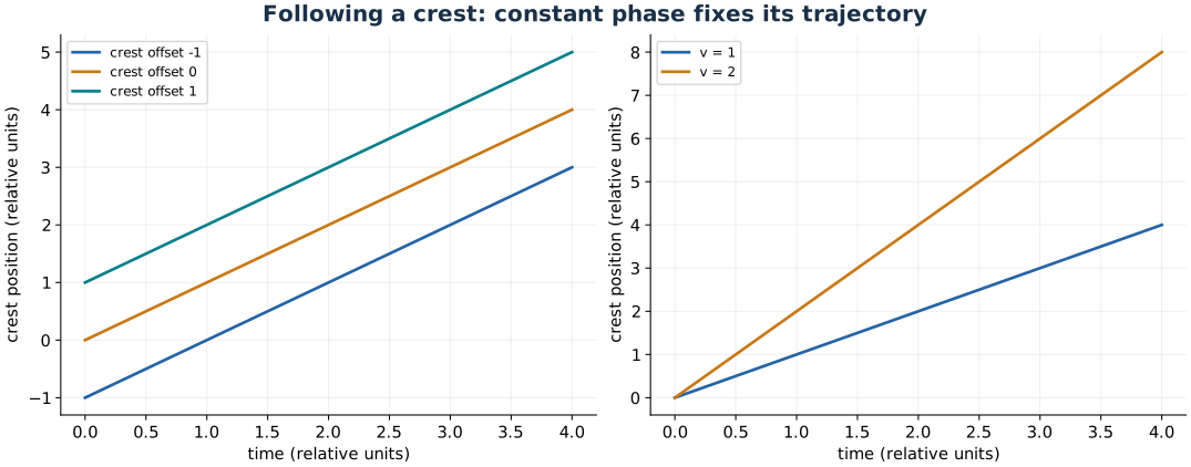
Constant-phase trajectories have slope equal to phase velocity. A larger phase offset shifts a crest without changing its speed.
Problem 1.48 — infer initial phase from a negative field maximum
Paraphrased task. Infer initial phase from a negative field maximum.
Formula reference. Use (3), its definitions, and the topic illustration.
Worked application.
Use \(E=20\sin(kx-\omega t+\phi_0)\,\mathrm{V/m}\).
At the origin and initial time, \(-20=20\sin\phi_0\), hence \(\sin\phi_0=-1\).
The sine reaches \(-1\) at \(3\pi/2\) modulo \(2\pi\). Equivalently use \(-\pi/2\); the cosine representation would require a different numerical phase.
Result. \(\phi_0=3\pi/2+2\pi m\), \(m\in\mathbb Z\), for the sine convention.
Check. Direct substitution gives \(E(0,0)=-20\,\mathrm{V/m}\).
Problem 1.49 — infer phase when the spatial origin is a maximum
Paraphrased task. Infer phase when the spatial origin is a maximum.
Formula reference. Use (3), its definitions, and the topic illustration.
Worked application.
A positive maximum at \(x=t=0\) means \(E(0,0)/E_0=1\).
In the sine representation this requires \(\sin\phi_0=1\); therefore \(\phi_0=\pi/2+2\pi m\).
Distinguish a positive maximum from a maximum absolute value: the latter also permits a negative crest, with phase \(3\pi/2\).
Result. \(\phi_0=\pi/2\pmod{2\pi}\) for a positive sine-wave maximum.
Check. The spatial derivative is zero at the crest and its second derivative is negative.
Problem 1.50 — describe phase evolution at a fixed observer
Paraphrased task. Describe phase evolution at a fixed observer.
Formula reference. Use (3), its definitions, and the topic illustration.
Worked application.
Choose the phase \(\Phi=kx-\omega t+\phi_0\) for motion toward positive \(x\).
At a fixed detector \(x=x_d\), the term \(kx_d+\phi_0\) is constant. Thus \(\Phi(t+\Delta t)-\Phi(t)=-\omega\Delta t\).
The unwrapped phase is a descending straight line. A phase instrument reporting modulo \(2\pi\) would show repeated wraps; these do not represent jumps in the physical field.
Result. \((\partial\Phi/\partial t)_x=-\omega\).
Check. In one period the unwrapped phase falls by \(2\pi\), while the field returns to its original value.
Problem 1.51 — describe phase variation across a snapshot
Paraphrased task. Describe phase variation across a snapshot.
Formula reference. Use (3), its definitions, and the topic illustration.
Worked application.
Freeze the time at \(t_0\); the phase is \(\Phi(x)=kx+(\phi_0-\omega t_0)\).
Two positions separated by \(\Delta x\) have phase difference \(\Delta\Phi=k\Delta x\).
Consequently the spatial slope is \(k\), and a distance \(\lambda=2\pi/k\) advances the phase by one full cycle. The diagram’s phase slope and wavelength encode the same information.
Result. \((\partial\Phi/\partial x)_t=k\).
Check. Position must be expressed in the same length units used to specify \(k\).
Problem 1.52 — find separations producing a sixty-degree phase offset
Paraphrased task. Find separations producing a sixty-degree phase offset.
Formula reference. Use (3), its definitions, and the topic illustration.
Worked application.
Calculate \(\lambda=c/f=(3\times10^8)/(3\times10^{14})=10^{-6}\,\mathrm m\).
The requested phase offset is \(60^\circ=\pi/3\). Since \(k\Delta x=\pi/3+2\pi m\), divide by \(k=2\pi/\lambda\).
This gives \(\Delta x=(m+1/6)\lambda\). For \(m=0,1,2\), the positive separations are 166.7, 1166.7, and 2166.7 nm. Reversing the ordering of the two points reverses the signed offset.
Result. \(\Delta x=(m+1/6)\,\mu\mathrm m\) for a signed \(+60^\circ\) phase difference modulo a cycle.
Check. The smallest positive separation is one sixth of a wavelength, not one sixth of a metre.
Problem 1.53 — count phase cycles and wave-train length
Paraphrased task. Count phase cycles and wave-train length.
Formula reference. Use (3), its definitions, and the topic illustration.
Worked application.
Convert \(500\,\mathrm{THz}=5.00\times10^{14}\,\mathrm{Hz}\) and a billionth of a second to \(\Delta t=10^{-9}\,\mathrm s\).
The number of cycles is \(N=f\Delta t=5.00\times10^5\); the phase-change magnitude is \(2\pi N=10^6\pi\,\mathrm{rad}\).
The associated train length is \(\ell=c\Delta t=0.300\,\mathrm m\). Independently, \(\lambda=c/f=600\,\mathrm{nm}\) and \(N\lambda=0.300\,\mathrm m\).
Result. A phase change of \(10^6\pi\) radians in magnitude and a 0.300 m train.
Check. Frequency times time counts cycles; multiplying by \(2\pi\) is needed to obtain radians.
Problem 1.54 — construct a wave from measured phase gradients
Paraphrased task. Construct a wave from measured phase gradients.
Formula reference. Use (3), its definitions, and the topic illustration.
Worked application.
The printed spatial gradient is \(k=4\pi\times10^6\,\mathrm{rad/m}\); the time-gradient magnitude is \(\omega=12\pi\times10^{14}\,\mathrm{rad/s}\).
Positive-x motion uses a negative time term. With amplitude 10 and initial phase \(\pi/3\), write
\[y=10\sin(4\pi10^6x-12\pi10^{14}t+\pi/3).\]Division gives \(v=\omega/k=3\times10^8\,\mathrm{m/s}\). The exponent on the spatial gradient is 6, not 8; the latter would contradict the stated speed.
Result. The displayed wave has \(v=3.0\times10^8\,\mathrm{m/s}\) toward positive \(x\).
Check. Differentiating its phase reproduces both measured gradients and \(y(0,0)=5\sqrt3\).
Complex-number representation
Formula and definitions.
Conjugation changes \(i\) to \(-i\) everywhere, including exponential phases. Euler’s identity converts \(Ae^{i\Phi}\) to \(A(\cos\Phi+i\sin\Phi)\). A physical squared field is \([\Re(Ae^{i\Phi})]^2=A^2\cos^2\Phi\), not merely the real part of \(zz^*\).
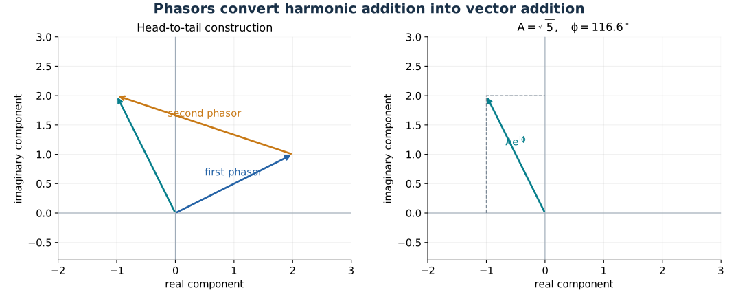
Complex amplitudes add as vectors. The resultant’s length and argument determine amplitude and phase.
Problem 1.55 — form complex conjugates
Paraphrased task. Form complex conjugates.
Formula reference. Use (4), its definitions, and the topic illustration.
Worked application.
Rationalize the first number: \((1-4i)/(2i)=-2-i/2\), so its conjugate is \(-2+i/2\).
Combine the phases in the second: \(2e^{i\omega t}e^{-ikx}=2e^{i(\omega t-kx)}\). Conjugation reverses the entire phase.
For the third, use \(1/(5i)=-i/5\) and \((4i)^2=-16\), giving \(16+i/20\). Its conjugate is therefore \(16-i/20\).
Result. The conjugates are \(-2+i/2\), \(2e^{-i(\omega t-kx)}\), and \(16-i/20\).
Check. Each original-plus-conjugate is twice a real number, and their products are nonnegative real numbers.
Problem 1.56 — extract real parts of phasors
Paraphrased task. Extract real parts of phasors.
Formula reference. Use (4), its definitions, and the topic illustration.
Worked application.
Multiply \((1-4i)/(2i)\) by \(-i/(-i)\) to obtain \(-2-i/2\).
Euler’s identity gives \(2e^{i(\omega t-kx)}=2\cos(\omega t-kx)+2i\sin(\omega t-kx)\).
Read the coefficients independent of \(i\); these, not the absolute values of the expressions, are the requested real parts.
Result. \(\Re z_1=-2\) and \(\Re z_2=2\cos(\omega t-kx)\).
Check. The real part can be negative; it must not be replaced by the complex magnitude.
Problem 1.57 — extract imaginary parts of phasors
Paraphrased task. Extract imaginary parts of phasors.
Formula reference. Use (4), its definitions, and the topic illustration.
Worked application.
Multiplying exponentials adds phases, so the first expression is \(5e^{i(kx+\omega t+\epsilon)}\).
Dividing the second pair subtracts the denominator’s phase, giving \((A/B)e^{i(\omega t-kx+\epsilon)}\) for real \(A,B\).
The symmetric pair is \((e^{i\omega t}+e^{-i\omega t})/2=\cos\omega t\); the opposite imaginary contributions cancel.
Result. The imaginary parts are \(5\sin(kx+\omega t+\epsilon)\), \((A/B)\sin(\omega t-kx+\epsilon)\), and zero.
Check. The imaginary part is the real coefficient multiplying \(i\), not that coefficient times \(i\).
Problem 1.58 — calculate phasor magnitudes
Paraphrased task. Calculate phasor magnitudes.
Formula reference. Use (4), its definitions, and the topic illustration.
Worked application.
A pure phase \(e^{i\Phi}\) has \(zz^*=1\); its magnitude is one.
Factor \(e^{iky}\) from the second expression, leaving \(2e^{i\omega t}+4e^{-i\omega t}\). The unit phase factor cannot change its magnitude.
Multiply by the conjugate and collect the cross terms:
\[|z|^2=4+16+8e^{2i\omega t}+8e^{-2i\omega t} =20+16\cos2\omega t.\]Take the positive square root only after combining the terms.
Result. The magnitudes are \(1\) and \(2\sqrt{5+4\cos2\omega t}\).
Check. The second magnitude ranges from \(|4-2|=2\) to \(4+2=6\), as required by vector addition.
Problem 1.59 — square a real harmonic field without confusing it with intensity
Paraphrased task. Square a real harmonic field without confusing it with intensity.
Formula reference. Use (4), its definitions, and the topic illustration.
Worked application.
Introduce \(z=Ae^{i\Phi}\) with \(\Phi=kx-\omega t\); the physical displacement is \(y=(z+z^*)/2\).
Square that real quantity:
\[y^2=\frac{z^2+2zz^*+(z^*)^2}{4} =\frac{A^2}{2}(1+\cos2\Phi)=A^2\cos^2\Phi.\]By contrast \(zz^*=A^2\) is constant. It contains amplitude information but omits the instantaneous oscillation. Time averaging the physical square gives \(A^2/2\).
Result. \(y^2=A^2\cos^2(kx-\omega t)\), whereas \(\langle y^2\rangle=A^2/2\).
Check. At a zero crossing the physical square vanishes although \(zz^*\) remains \(A^2\).
Three-dimensional waves
Formula and definitions.
Write \(\mathbf k=k\hat{\mathbf s}\), where the supplied direction is normalized to unit length. The chain rule gives \(\nabla^2 f(\Phi)=k^2f''(\Phi)\) and \(\partial_t^2f(\Phi)=\omega^2f''(\Phi)\), proving the 3-D wave equation when \(\omega=vk\).
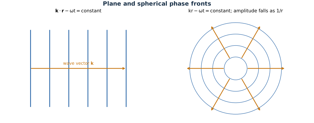
Parallel phase planes describe a plane wave; concentric phase circles are sections of spherical wavefronts.
Problem 1.60 — verify an arbitrary three-dimensional plane-wave profile
Paraphrased task. Verify an arbitrary three-dimensional plane-wave profile.
Formula reference. Use (5), its definitions, and the topic illustration.
Worked application.
Let \(u=k(\alpha x+\beta y+\gamma z)-\omega t\), with unit direction cosines satisfying \(\alpha^2+\beta^2+\gamma^2=1\).
The three second spatial derivatives are \(k^2\alpha^2f''\), \(k^2\beta^2f''\), and \(k^2\gamma^2f''\); summing gives \(\nabla^2f=k^2f''\).
The time derivative is \(f_{tt}=\omega^2f''\). Thus \(\nabla^2f=f_{tt}/v^2\) precisely when \(\omega^2=v^2k^2\). Constant-phase surfaces are planes normal to \((\alpha,\beta,\gamma)\).
Result. Every twice-differentiable profile of this form is a plane wave when \(\omega=vk\).
Check. If the direction vector is not normalized, its norm must be included in the magnitude of the wavevector.
Problem 1.61 — write a wave along the diagonal in the xy plane
Paraphrased task. Write a wave along the diagonal in the xy plane.
Formula reference. Use (5), its definitions, and the topic illustration.
Worked application.
The supplied direction \(\hat{\mathbf s}=(\hat{\mathbf x}+\hat{\mathbf y})/\sqrt2\) is already normalized.
Form \(\mathbf k=(2\pi/\lambda)\hat{\mathbf s}\), so \(\mathbf k\cdot\mathbf r=2\pi(x+y)/(\lambda\sqrt2)\).
Insert \(\omega=2\pi v/\lambda\) and choose an arbitrary phase origin, for example zero. Translation along \(\hat{\mathbf s}\) by \(\lambda\) adds exactly \(2\pi\).
Result. \(\psi=A\sin[2\pi(x+y)/(\lambda\sqrt2)-2\pi vt/\lambda]\).
Check. The component wavelengths along the coordinate axes are \(\sqrt2\lambda\); the wavelength along propagation is \(\lambda\).
Problem 1.62 — identify the constant-time phase gradient
Paraphrased task. Identify the constant-time phase gradient.
Formula reference. Use (5), its definitions, and the topic illustration.
Worked application.
Write \(\Phi=k_xx+k_yy+k_zz-\omega t+\phi_0\).
At constant time, its partial derivatives are respectively \(k_x,k_y,k_z\).
Assemble the gradient:
\[\nabla\Phi=k_x\hat{\mathbf x}+k_y\hat{\mathbf y}+k_z\hat{\mathbf z}=\mathbf k.\]A displacement tangent to a wavefront has \(\mathbf k\cdot d\mathbf r=0\), explaining why this vector is normal to the wavefront.
Result. \((\nabla\Phi)_t=\mathbf k\) with magnitude \(2\pi/\lambda\).
Check. The gradient has units radians per metre and points toward increasing spatial phase.
Problem 1.63 — normalize a propagation-direction vector
Paraphrased task. Normalize a propagation-direction vector.
Formula reference. Use (5), its definitions, and the topic illustration.
Worked application.
Read the three spatial coefficients from the phase: \(\mathbf k=k(1,-2,3)/\sqrt{14}\).
Its norm is \(k\sqrt{1+4+9}/\sqrt{14}=k\). Divide the coefficient vector by this norm.
Since the time term is \(-\omega t\), the constant-phase surfaces advance along this vector, not its negative.
Result. \(\hat{\mathbf s}=(\hat{\mathbf x}-2\hat{\mathbf y}+3\hat{\mathbf z})/\sqrt{14}\).
Check. The direction cosines have squared sum one; the negative y component must survive normalization.
Problem 1.64 — write a Cartesian plane wave through a specified direction point
Paraphrased task. Write a cartesian plane wave through a specified direction point.
Formula reference. Use (5), its definitions, and the topic illustration.
Worked application.
The direction from the origin through \((2,2,3)\) has length \(\sqrt{2^2+2^2+3^2}=\sqrt{17}\).
Normalize it and multiply by \(k=2\pi/\lambda\): \(\mathbf k=(2\pi/\lambda)(2,2,3)/\sqrt{17}\).
Take the dot product with the observation coordinate and use the negative time sign for outward propagation. An arbitrary initial phase can be added without changing the direction.
Result. \(\psi=A\sin[2\pi(2x+2y+3z)/(\lambda\sqrt{17})-\omega t+\phi_0]\).
Check. Putting \(\mathbf r=\ell(2,2,3)/\sqrt{17}\) reduces the phase to \(k\ell-\omega t+\phi_0\).