Chapter 7: Photonic-Crystal Optics
Source: Saleh and Teich, Fundamentals of Photonics, second edition, Chapter 7. The characteristic-matrix convention is the book’s.
In-text exercise
Exercise 7.1-1 — Quarter-wave antireflection film
Brief solution
1. Method. The working uses matrix multiplication and eigenvalue rules, trigonometric and small-angle identities, and algebraic rearrangement and dimensional checks.
Show detailed steps
Step 1 — Definitions and setup. Symbols are local to this item and follow the chapter convention. Each physical quantity and supplied numerical value is introduced at its first use below; angles are in radians unless a degree symbol is shown, and units are retained through numerical substitution.
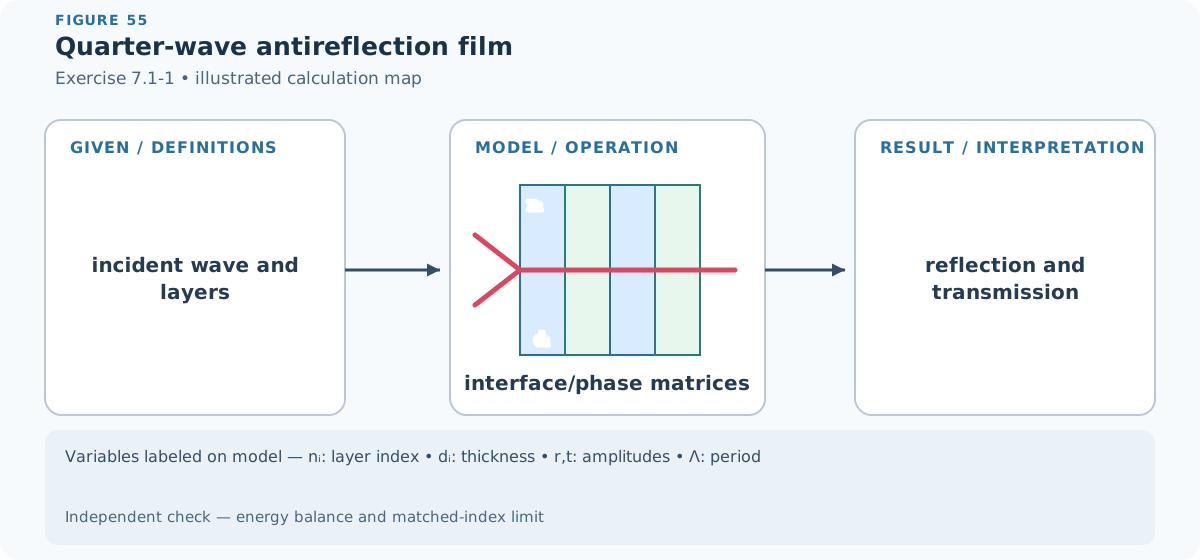
Figure 55 — Exercise 7.1-1: Quarter-wave antireflection film. The diagram identifies the input quantities, physical operation, requested result, variable meanings, and an independent verification route. Every symbol in the variable strip is labeled on the model itself.
Step 2 — Mathematical formulas used. The working uses matrix multiplication and eigenvalue rules, trigonometric and small-angle identities, and algebraic rearrangement and dimensional checks.
Step 3 — Worked derivation. The calculation is kept in symbolic form until the governing relation has been rearranged for the requested quantity.
Detailed step 1. Multiplying boundary/propagation matrices makes \(B\propto n_1n_3\sin^2\delta-n_2^2\sin^2\delta\) at \(\delta=\pi/2\).
Detailed step 2. Thus \(B=0\) and \(r=0\) when \(\boxed{d=\lambda_0/(4n_2),\ n_2=\sqrt{n_1n_3}}\).
End-of-chapter problems
Step 4 — State the numbered result. The principal result obtained in the working is
Step 5 — Check. Equation (1) can be checked by substituting it back into the preceding governing relation and reversing the algebraic steps. Multiply the matrices independently in the stated input-to-output order and verify that every product has compatible dimensions.
Problem 7.1-2 — Slab beamsplitter
Brief solution
1. Method. The working uses trigonometric and small-angle identities and algebraic rearrangement and dimensional checks.
2. Reasoning and answer.
Show detailed steps
Definitions and setup. Symbols are local to this item and follow the chapter convention. Each physical quantity and supplied numerical value is introduced at its first use below; angles are in radians unless a degree symbol is shown, and units are retained through numerical substitution.
Mathematical formulas used. The working uses trigonometric and small-angle identities and algebraic rearrangement and dimensional checks.
Worked derivation. The calculation is kept in symbolic form until the governing relation has been rearranged for the requested quantity.
Detailed step 1. Use the Airy result \(T=[1+4R_{s,p}\sin^2\delta/(1-R_{s,p})^2]^{-1}\), \(R=1-T\),
Detailed step 2. with the TE/TM Fresnel \(R_{s,p}\) at 45 degrees and \(\delta=(2\pi/\lambda_0)nd\cos\theta_t\).
Detailed step 3. This directly supplies the periodic spectral curves;
Detailed step 4. TM contrast vanishes when the internal/external angle is Brewster.
Numbered result. The principal result obtained in the working is
Check. Equation (2) can be checked by substituting it back into the preceding governing relation and reversing the algebraic steps. The zero-angle or paraxial limit supplies an independent sign and magnitude check whenever that limit is part of the model.
Problem 7.1-3 — Air-gap tunnelling
Brief solution
1. Method. The working uses matrix multiplication and eigenvalue rules, trigonometric and small-angle identities, and algebraic rearrangement and dimensional checks.
2. Reasoning and answer.
Show detailed steps
Definitions and setup. Symbols are local to this item and follow the chapter convention. Each physical quantity and supplied numerical value is introduced at its first use below; angles are in radians unless a degree symbol is shown, and units are retained through numerical substitution.
Mathematical formulas used. The working uses matrix multiplication and eigenvalue rules, trigonometric and small-angle identities, and algebraic rearrangement and dimensional checks.
Worked derivation. The calculation is kept in symbolic form until the governing relation has been rearranged for the requested quantity.
Detailed step 1. At normal incidence insert \(n_g,1,n_g\) in the slab matrix and \(d=\lambda_0/2\); the round-trip phase gives unity transmission.
Detailed step 2. Above critical angle the gap normal wavevector is \(j\kappa\); replacing \(\sin\delta,j\cos\delta\) by hyperbolic functions gives finite \(T\propto\operatorname{sech}^2(\kappa d)\): frustrated TIR tunnels through a sufficiently thin gap.
Numbered result. The principal result obtained in the working is
Check. Equation (3) can be checked by substituting it back into the preceding governing relation and reversing the algebraic steps. Multiply the matrices independently in the stated input-to-output order and verify that every product has compatible dimensions.
Problem 7.1-4 — Unmatched incident medium
Brief solution
1. Method. The working uses algebraic rearrangement and dimensional checks.
2. Reasoning and answer.
Show detailed steps
Definitions and setup. Symbols are local to this item and follow the chapter convention. Each physical quantity and supplied numerical value is introduced at its first use below; angles are in radians unless a degree symbol is shown, and units are retained through numerical substitution.
Mathematical formulas used. The working uses algebraic rearrangement and dimensional checks.
Worked derivation. The calculation is kept in symbolic form until the governing relation has been rearranged for the requested quantity.
Detailed step 1. Composition of the new boundary and old device gives \(\boxed{r=(r_b+r_m)/(1+r_br_m)}\).
Detailed step 2. It reduces respectively to \(r_m,1,r_b,1\) for \(r_b=0,1\) and \(r_m=0,1\).
Numbered result. The principal result obtained in the working is
Check. Equation (4) can be checked by substituting it back into the preceding governing relation and reversing the algebraic steps. Check that dimensions agree term by term, then test the simplest symmetry or limiting case for the expected sign and scale.
Problem 7.1-5 — Oblique quarter-wave coating
Brief solution
1. Method. The working uses matrix multiplication and eigenvalue rules, exponential, logarithmic, and phasor identities, and trigonometric and small-angle identities.
2. Reasoning and answer.
Show detailed steps
Definitions and setup. Symbols are local to this item and follow the chapter convention. Each physical quantity and supplied numerical value is introduced at its first use below; angles are in radians unless a degree symbol is shown, and units are retained through numerical substitution.
Mathematical formulas used. The working uses matrix multiplication and eigenvalue rules, exponential, logarithmic, and phasor identities, and trigonometric and small-angle identities.
Worked derivation. The calculation is kept in symbolic form until the governing relation has been rearranged for the requested quantity.
Detailed step 1. Replace admittance by \(n\cos\theta\) (TE) or \(n/\cos\theta\) (TM),
Detailed step 2. and phase by \(\delta=2\pi n_2d\cos\theta_2/\lambda_0\); multiplying the one-film matrix gives \(r=(r_{12}+r_{23}e^{-j2\delta})/ (1+r_{12}r_{23}e^{-j2\delta})\).
Detailed step 3. Squaring this expression is the requested angular reflectance.
Numbered result. The principal result obtained in the working is
Check. Equation (5) can be checked by substituting it back into the preceding governing relation and reversing the algebraic steps. Multiply the matrices independently in the stated input-to-output order and verify that every product has compatible dimensions.
Problem 7.1-6 — Quarter/half-wave stacks
Brief solution
1. Method. The working uses matrix multiplication and eigenvalue rules and algebraic rearrangement and dimensional checks.
2. Reasoning and answer.
Show detailed steps
Definitions and setup. Symbols are local to this item and follow the chapter convention. Each physical quantity and supplied numerical value is introduced at its first use below; angles are in radians unless a degree symbol is shown, and units are retained through numerical substitution.
Mathematical formulas used. The working uses matrix multiplication and eigenvalue rules and algebraic rearrangement and dimensional checks.
Worked derivation. The calculation is kept in symbolic form until the governing relation has been rearranged for the requested quantity.
Detailed step 1. At the design wavelength a quarter-wave pair has diagonal matrix \(-\operatorname{diag}(n_2/n_1,n_1/n_2)\); after \(N\) pairs the ratio is raised to \(N\),
Detailed step 2. yielding \(r=[n_a(n_2/n_1)^{2N}-n_s]/[n_a(n_2/n_1)^{2N}+n_s]\) up to layer order.
Detailed step 3. A half-wave layer is \(-I\); every pair is transparent at the design wavelength apart from phase,
Detailed step 4. so only the unmatched outer boundary remains.
Numbered result. The principal result obtained in the working is
Check. Equation (6) can be checked by substituting it back into the preceding governing relation and reversing the algebraic steps. Multiply the matrices independently in the stated input-to-output order and verify that every product has compatible dimensions.
Problem 7.1-7 — GaAs/AlAs reflector
Brief solution
1. Method. The working uses algebraic rearrangement and dimensional checks.
2. Reasoning and answer.
Show detailed steps
Definitions and setup. Symbols are local to this item and follow the chapter convention. Each physical quantity and supplied numerical value is introduced at its first use below; angles are in radians unless a degree symbol is shown, and units are retained through numerical substitution.
Mathematical formulas used. The working uses algebraic rearrangement and dimensional checks.
Worked derivation. The calculation is kept in symbolic form until the governing relation has been rearranged for the requested quantity.
Detailed step 1. For a GaAs-matched exterior,
Detailed step 2. evaluate the preceding quarter-wave expression with \(n_1=3.57\), \(n_2=2.94\): \(\boxed{R_N=[(1-(n_2/n_1)^{2N})/(1+(n_2/n_1)^{2N})]^2}\) and \(T_N=1-R_N\).
Detailed step 3. Evaluating \(N=1,\ldots,10\) gives the requested monotonic plot.
Numbered result. The principal result obtained in the working is
Check. Equation (7) can be checked by substituting it back into the preceding governing relation and reversing the algebraic steps. Check that dimensions agree term by term, then test the simplest symmetry or limiting case for the expected sign and scale.
Problem 7.1-8 — Matrix-program verification
Brief solution
1. Method. The working uses matrix multiplication and eigenvalue rules, trigonometric and small-angle identities, and algebraic rearrangement and dimensional checks.
2. Reasoning and answer.
Show detailed steps
Definitions and setup. Symbols are local to this item and follow the chapter convention. Each physical quantity and supplied numerical value is introduced at its first use below; angles are in radians unless a degree symbol is shown, and units are retained through numerical substitution.
Mathematical formulas used. The working uses matrix multiplication and eigenvalue rules, trigonometric and small-angle identities, and algebraic rearrangement and dimensional checks.
Worked derivation. The calculation is kept in symbolic form until the governing relation has been rearranged for the requested quantity.
Detailed step 1. Initialize \(M=I\); for each layer multiply \(M_i=\begin{bmatrix}\cos\delta_i&j\sin\delta_i/Y_i\\ jY_i\sin\delta_i&\cos\delta_i\end{bmatrix}\).
Detailed step 2. Convert total input admittance to \(r\) and plot \(|r|^2\) versus wavelength or angle.
Detailed step 3. Using the figure’s layer data reproduces its stopband and TE/TM angular splitting.
Numbered result. The principal result obtained in the working is
Check. Equation (8) can be checked by substituting it back into the preceding governing relation and reversing the algebraic steps. Multiply the matrices independently in the stated input-to-output order and verify that every product has compatible dimensions.
Problem 7.2-1 — Gap/midgap estimate
Brief solution
1. Method. The working uses trigonometric and small-angle identities and algebraic rearrangement and dimensional checks.
2. Reasoning and answer.
Show detailed steps
Definitions and setup. Symbols are local to this item and follow the chapter convention. Each physical quantity and supplied numerical value is introduced at its first use below; angles are in radians unless a degree symbol is shown, and units are retained through numerical substitution.
Mathematical formulas used. The working uses trigonometric and small-angle identities and algebraic rearrangement and dimensional checks.
Worked derivation. The calculation is kept in symbolic form until the governing relation has been rearranged for the requested quantity.
Detailed step 1. Equal optical thickness gives Bragg frequency \(\boxed{\nu_B=c/[2(n_1d_1+n_2d_2)]}\) with \(d_1+d_2=2\ \mathrm{\mu m}\).
Detailed step 2. The first-order relative gap is \(\Delta\nu/\nu_B\simeq(4/\pi)\sin^{-1}|(n_2-n_1)/(n_2+n_1)|\).
Detailed step 3. It is large for 1.5/3.5 and small for 3.4/3.6,
Detailed step 4. demonstrating that index contrast,
Detailed step 5. not mean index,
Detailed step 6. controls the fractional gap.
Numbered result. The principal result obtained in the working is
Check. Equation (9) can be checked by substituting it back into the preceding governing relation and reversing the algebraic steps. The zero-angle or paraxial limit supplies an independent sign and magnitude check whenever that limit is part of the model. Repeat the substitution with unrounded intermediate values and retain the displayed units; the final unit must have the requested dimension.
Problem 7.2-2 — Off-axis Bloch wave
Brief solution
1. Method. The working uses trigonometric and small-angle identities and algebraic rearrangement and dimensional checks.
2. Reasoning and answer.
Show detailed steps
Definitions and setup. Symbols are local to this item and follow the chapter convention. Each physical quantity and supplied numerical value is introduced at its first use below; angles are in radians unless a degree symbol is shown, and units are retained through numerical substitution.
Mathematical formulas used. The working uses trigonometric and small-angle identities and algebraic rearrangement and dimensional checks.
Worked derivation. The calculation is kept in symbolic form until the governing relation has been rearranged for the requested quantity.
Detailed step 1. Keep conserved \(k_x\); in every layer replace \(n_i\omega/c\) by \(k_{zi}=[(n_i\omega/c)^2-k_x^2]^{1/2}\) and admittance by its TE/TM oblique value.
Detailed step 2. The unit-cell trace then gives \(\boxed{\cos(K\Lambda)=\tfrac12\operatorname{tr}M(k_x,\omega)}\); \(|\operatorname{tr}M/2|>1\) is a bandgap.
Numbered result. The principal result obtained in the working is
Check. Equation (10) can be checked by substituting it back into the preceding governing relation and reversing the algebraic steps. The zero-angle or paraxial limit supplies an independent sign and magnitude check whenever that limit is part of the model.
Problem 7.2-3 — Propagation normal to periodicity
Brief solution
1. Method. The working uses algebraic rearrangement and dimensional checks.
2. Reasoning and answer.
Show detailed steps
Definitions and setup. Symbols are local to this item and follow the chapter convention. Each physical quantity and supplied numerical value is introduced at its first use below; angles are in radians unless a degree symbol is shown, and units are retained through numerical substitution.
Mathematical formulas used. The working uses algebraic rearrangement and dimensional checks.
Worked derivation. The calculation is kept in symbolic form until the governing relation has been rearranged for the requested quantity.
Detailed step 1. For \(K=0\) (wavevector along the layers),
Detailed step 2. tangential phase matching makes the field sample a translationally uniform direction.
Detailed step 3. Substitution in the off-axis dispersion relation leaves real \(k_x\) for every allowed frequency; the Bragg coupling term vanishes,
Detailed step 4. so no axial-period bandgap opens.
Numbered result. The principal result obtained in the working is
Check. Equation (11) can be checked by substituting it back into the preceding governing relation and reversing the algebraic steps. Check that dimensions agree term by term, then test the simplest symmetry or limiting case for the expected sign and scale.
Problem 7.2-4 — Omnidirectional reflector
Brief solution
1. Method. The working uses algebraic rearrangement and dimensional checks.
2. Reasoning and answer.
Show detailed steps
Definitions and setup. Symbols are local to this item and follow the chapter convention. Each physical quantity and supplied numerical value is introduced at its first use below; angles are in radians unless a degree symbol is shown, and units are retained through numerical substitution.
Mathematical formulas used. The working uses algebraic rearrangement and dimensional checks.
Worked derivation. The calculation is kept in symbolic form until the governing relation has been rearranged for the requested quantity.
Detailed step 1. For each conserved air \(k_x\leq\omega/c\),
Detailed step 2. evaluate the cell trace with \(n_2=2n_1\) and equal optical thickness.
Detailed step 3. Shade frequencies for which \(|\operatorname{tr}M/2|>1\) for every point inside the air light cone; the intersection of all angular TE/TM stopbands is the omnidirectional range.
Detailed step 4. This construction,
Detailed step 5. rather than a single normal-incidence gap,
Detailed step 6. is the required projected dispersion plot.
Numbered result. The principal result obtained in the working is
Check. Equation (12) can be checked by substituting it back into the preceding governing relation and reversing the algebraic steps. Check that dimensions agree term by term, then test the simplest symmetry or limiting case for the expected sign and scale.