Chapter 20: Electro-Optics

Source: Saleh and Teich, Fundamentals of Photonics, second edition, Chapter 20.

In-text exercises

Exercise 20.1-1 — Directional-coupler spectral response

Brief solution

1. Method. The working uses trigonometric and small-angle identities and algebraic rearrangement and dimensional checks.

2. Key step.

Since \(V_0(\lambda)=V_0(\lambda_r)\lambda/\lambda_r\), holding \(V=V_0(\lambda_r)\) gives coupling phase \((\pi/2)(\lambda_r/\lambda)\). Therefore

3. Answer.

\[\boxed{\eta(\lambda)=\cos^2\!\left({\pi\lambda_r\over2\lambda}\right)}.\]

It has a quadratic null at \(\lambda_r\); this expression directly generates the requested wavelength-detuning plot.

Show detailed stepsHide detailed steps

Step 1 — Definitions and setup. Symbols are local to this item and follow the chapter convention. Each physical quantity and supplied numerical value is introduced at its first use below; angles are in radians unless a degree symbol is shown, and units are retained through numerical substitution.

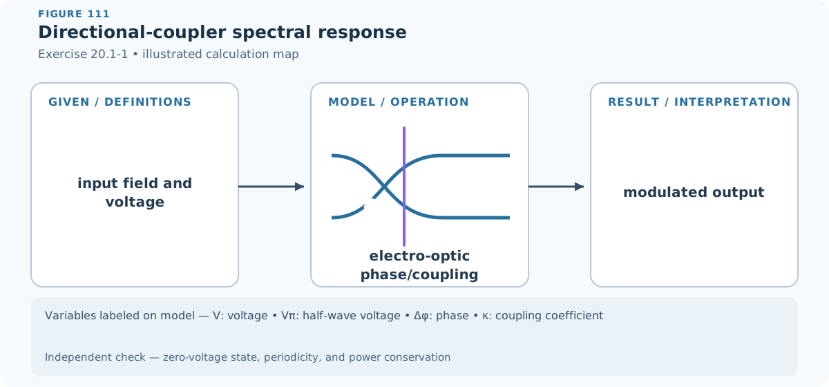
Figure 111 — Exercise 20.1-1: Directional-coupler spectral response. The diagram identifies the input quantities, physical operation, requested result, variable meanings, and an independent verification route. Every symbol in the variable strip is labeled on the model itself.

Step 2 — Mathematical formulas used. The working uses trigonometric and small-angle identities and algebraic rearrangement and dimensional checks.

Step 3 — Worked derivation. The calculation is kept in symbolic form until the governing relation has been rearranged for the requested quantity.

Since \(V_0(\lambda)=V_0(\lambda_r)\lambda/\lambda_r\), holding \(V=V_0(\lambda_r)\) gives coupling phase \((\pi/2)(\lambda_r/\lambda)\). Therefore

(1)\[\boxed{\eta(\lambda)=\cos^2\!\left({\pi\lambda_r\over2\lambda}\right)}.\]

It has a quadratic null at \(\lambda_r\); this expression directly generates the requested wavelength-detuning plot.

Step 4 — Interpret the result. The final relation or conclusion in Step 3 is the requested result. Read its sign, scale, or physical classification using the conventions fixed in Step 1.

Step 5 — Check. Equation (1) can be checked by substituting it back into the preceding governing relation and reversing the algebraic steps. The zero-angle or paraxial limit supplies an independent sign and magnitude check whenever that limit is part of the model. Repeat the substitution with unrounded intermediate values and retain the displayed units; the final unit must have the requested dimension.

Exercise 20.2-1 — Longitudinal Kerr modulation

Brief solution

1. Method. The working uses exponential, logarithmic, and phasor identities and algebraic rearrangement and dimensional checks.

2. Key step.

For eigenpolarization \(i\), \(n_i(E)\simeq n_i-s_i n_i^3E^2/2\). With \(E=V/L\),

\[\phi_i=\phi_{i0}-{\pi s_i n_i^3\over\lambda_0 L}V^2, \qquad \Gamma=\Gamma_0-{\pi(s_xn_x^3-s_yn_y^3)\over\lambda_0L}V^2.\]

3. Answer.

Setting the voltage-induced phase or retardation magnitude to \(\pi\) gives \(\boxed{V_\pi=\sqrt{\lambda_0L/(|s|n^3)}}\), with \(s n^3\) replaced by the eigenpolarization difference for a retarder.

Show detailed stepsHide detailed steps

Step 1 — Definitions and setup. Symbols are local to this item and follow the chapter convention. Each physical quantity and supplied numerical value is introduced at its first use below; angles are in radians unless a degree symbol is shown, and units are retained through numerical substitution.

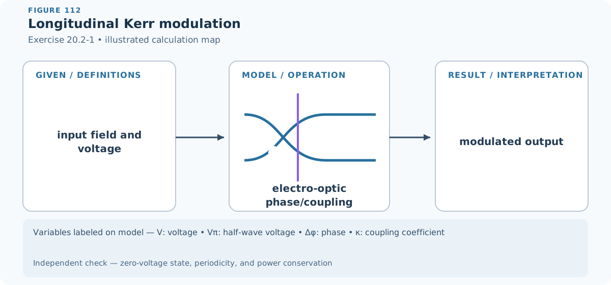
Figure 112 — Exercise 20.2-1: Longitudinal Kerr modulation. The diagram identifies the input quantities, physical operation, requested result, variable meanings, and an independent verification route. Every symbol in the variable strip is labeled on the model itself.

Step 2 — Mathematical formulas used. The working uses exponential, logarithmic, and phasor identities and algebraic rearrangement and dimensional checks.

Step 3 — Worked derivation. The calculation is kept in symbolic form until the governing relation has been rearranged for the requested quantity.

For eigenpolarization \(i\), \(n_i(E)\simeq n_i-s_i n_i^3E^2/2\). With \(E=V/L\),

(2)\[\phi_i=\phi_{i0}-{\pi s_i n_i^3\over\lambda_0 L}V^2, \qquad \Gamma=\Gamma_0-{\pi(s_xn_x^3-s_yn_y^3)\over\lambda_0L}V^2.\]

Setting the voltage-induced phase or retardation magnitude to \(\pi\) gives \(\boxed{V_\pi=\sqrt{\lambda_0L/(|s|n^3)}}\), with \(s n^3\) replaced by the eigenpolarization difference for a retarder.

End-of-chapter problems

Step 4 — Interpret the result. The final relation or conclusion in Step 3 is the requested result. Read its sign, scale, or physical classification using the conventions fixed in Step 1.

Step 5 — Check. Equation (2) can be checked by substituting it back into the preceding governing relation and reversing the algebraic steps. Check that dimensions agree term by term, then test the simplest symmetry or limiting case for the expected sign and scale. Repeat the substitution with unrounded intermediate values and retain the displayed units; the final unit must have the requested dimension.

Problem 20.1-2 — GaAs phase-modulator speed

Brief solution

1. Method. The working uses algebraic rearrangement and dimensional checks.

2. Reasoning and answer.

\[\epsilon A/L=\boxed{0.398\ \mathrm{pF}}\]

Show detailed stepsHide detailed steps

Definitions and setup. Symbols are local to this item and follow the chapter convention. Each physical quantity and supplied numerical value is introduced at its first use below; angles are in radians unless a degree symbol is shown, and units are retained through numerical substitution.

Mathematical formulas used. The working uses algebraic rearrangement and dimensional checks.

Worked derivation. The calculation is kept in symbolic form until the governing relation has been rearranged for the requested quantity.

Detailed step 1. For a longitudinal cell, \(V_\pi=\lambda_0/(2rn^3)=\boxed{8.71\ \mathrm{kV}}\) and the optical transit time is \(nL/c=\boxed{0.360\ \mathrm{ns}}\).

Detailed step 2. The parallel-plate capacitance is \(\epsilon A/L=\boxed{0.398\ \mathrm{pF}}\),

Detailed step 3. so the 50-ohm time constant is only \(19.9\) ps.

Detailed step 4. Optical transit,

Detailed step 5. not the RC circuit,

Detailed step 6. is the limiting scale.

Numbered result. The principal result obtained in the working is

(3)\[\epsilon A/L=\boxed{0.398\ \mathrm{pF}}\]

Check. Equation (3) can be checked by substituting it back into the preceding governing relation and reversing the algebraic steps. Check that dimensions agree term by term, then test the simplest symmetry or limiting case for the expected sign and scale. Repeat the substitution with unrounded intermediate values and retain the displayed units; the final unit must have the requested dimension.

Problem 20.1-3 — Mach–Zehnder sensitivity

Brief solution

1. Method. The working uses stationary-value condition, product, quotient, and chain rules, and trigonometric and small-angle identities.

2. Reasoning and answer.

\[\boxed{|d\eta/dV|_{max}=\pi/(2V_\pi)=0.1571\ \mathrm{V^{-1}}}\]

Show detailed stepsHide detailed steps

Definitions and setup. Symbols are local to this item and follow the chapter convention. Each physical quantity and supplied numerical value is introduced at its first use below; angles are in radians unless a degree symbol is shown, and units are retained through numerical substitution.

Mathematical formulas used. The working uses stationary-value condition, product, quotient, and chain rules, and trigonometric and small-angle identities.

Worked derivation. The calculation is kept in symbolic form until the governing relation has been rearranged for the requested quantity.

Detailed step 1. Bias at quadrature,

Detailed step 2. where \(\eta=[1+\cos(\pi V/V_\pi)]/2\) has maximum slope.

Detailed step 3. Thus \(\boxed{|d\eta/dV|_{max}=\pi/(2V_\pi)=0.1571\ \mathrm{V^{-1}}}\) for \(V_\pi=10\) V.

Numbered result. The principal result obtained in the working is

(4)\[\boxed{|d\eta/dV|_{max}=\pi/(2V_\pi)=0.1571\ \mathrm{V^{-1}}}\]

Check. Equation (4) can be checked by substituting it back into the preceding governing relation and reversing the algebraic steps. The zero-angle or paraxial limit supplies an independent sign and magnitude check whenever that limit is part of the model. Repeat the substitution with unrounded intermediate values and retain the displayed units; the final unit must have the requested dimension.

Problem 20.1-4 — Integrated strain sensor

Brief solution

1. Method. The working uses product, quotient, and chain rules, integration identities, and algebraic rearrangement and dimensional checks.

2. Reasoning and answer.

\[\boxed{\epsilon=n^3rV/[2d(\partial n/\partial\epsilon)]}\]

Show detailed stepsHide detailed steps

Definitions and setup. Symbols are local to this item and follow the chapter convention. Each physical quantity and supplied numerical value is introduced at its first use below; angles are in radians unless a degree symbol is shown, and units are retained through numerical substitution.

Mathematical formulas used. The working uses product, quotient, and chain rules, integration identities, and algebraic rearrangement and dimensional checks.

Worked derivation. The calculation is kept in symbolic form until the governing relation has been rearranged for the requested quantity.

Detailed step 1. Put the sensing and reference waveguides in a Mach–Zehnder and bias it at quadrature.

Detailed step 2. Strain produces \(\Delta\phi_s=k_0L(\partial n/\partial \epsilon)\epsilon\).

Detailed step 3. Apply a feedback voltage giving \(\Delta\phi_E=-k_0Ln^3rV/(2d)\) and servo the detector back to its null; then \(\boxed{\epsilon=n^3rV/[2d(\partial n/\partial\epsilon)]}\).

Detailed step 4. The null measurement removes source-power drift.

Numbered result. The principal result obtained in the working is

(5)\[\boxed{\epsilon=n^3rV/[2d(\partial n/\partial\epsilon)]}\]

Check. Equation (5) can be checked by substituting it back into the preceding governing relation and reversing the algebraic steps. Differentiation of an antiderivative, or normalization of a definite integral, checks the integration step.

Problem 20.1-5 — Faraday intensity modulation

Brief solution

1. Method. The working uses trigonometric and small-angle identities and algebraic rearrangement and dimensional checks.

2. Reasoning and answer.

\[\boxed{I_o/I_i=\cos^2[\alpha+V_B B(t)L]}\]

Show detailed stepsHide detailed steps

Definitions and setup. Symbols are local to this item and follow the chapter convention. Each physical quantity and supplied numerical value is introduced at its first use below; angles are in radians unless a degree symbol is shown, and units are retained through numerical substitution.

Mathematical formulas used. The working uses trigonometric and small-angle identities and algebraic rearrangement and dimensional checks.

Worked derivation. The calculation is kept in symbolic form until the governing relation has been rearranged for the requested quantity.

Detailed step 1. Place the rotator between linear polarizers.

Detailed step 2. If their relative angle is \(\alpha\),

Detailed step 3. Malus’ law gives \(\boxed{I_o/I_i=\cos^2[\alpha+V_B B(t)L]}\).

Detailed step 4. Biasing at 45 degrees makes small field changes linear in output intensity; crossed polarizers instead make an on/off switch.

Numbered result. The principal result obtained in the working is

(6)\[\boxed{I_o/I_i=\cos^2[\alpha+V_B B(t)L]}\]

Check. Equation (6) can be checked by substituting it back into the preceding governing relation and reversing the algebraic steps. The zero-angle or paraxial limit supplies an independent sign and magnitude check whenever that limit is part of the model.

Problem 20.2-2 — Poled-silica phase shift

Brief solution

1. Method. The working uses algebraic rearrangement and dimensional checks.

2. Reasoning and answer.

\[\boxed{\Delta\phi=-0.3058\ \mathrm{rad}}\]

Show detailed stepsHide detailed steps

Definitions and setup. Symbols are local to this item and follow the chapter convention. Each physical quantity and supplied numerical value is introduced at its first use below; angles are in radians unless a degree symbol is shown, and units are retained through numerical substitution.

Mathematical formulas used. The working uses algebraic rearrangement and dimensional checks.

Worked derivation. The calculation is kept in symbolic form until the governing relation has been rearranged for the requested quantity.

Detailed step 1. For the stated axes and \(y\) polarization, \(r_{13}\) applies.

Detailed step 2. Substitution in \(\Delta\phi=-\pi r n^3(V/d)L/\lambda\) gives \(\boxed{\Delta\phi=-0.3058\ \mathrm{rad}}\) (magnitude 17.5 degrees).

Numbered result. The principal result obtained in the working is

(7)\[\boxed{\Delta\phi=-0.3058\ \mathrm{rad}}\]

Check. Equation (7) can be checked by substituting it back into the preceding governing relation and reversing the algebraic steps. Check that dimensions agree term by term, then test the simplest symmetry or limiting case for the expected sign and scale. Repeat the substitution with unrounded intermediate values and retain the displayed units; the final unit must have the requested dimension.

Problem 20.2-3 — Cascaded KDP cells

Brief solution

1. Method. The working uses trigonometric and small-angle identities and algebraic rearrangement and dimensional checks.

2. Reasoning and answer.

\[\boxed{V_{\pi,9}=V_\pi/9=1.87\ \mathrm{kV}}\]

Show detailed stepsHide detailed steps

Definitions and setup. Symbols are local to this item and follow the chapter convention. Each physical quantity and supplied numerical value is introduced at its first use below; angles are in radians unless a degree symbol is shown, and units are retained through numerical substitution.

Mathematical formulas used. The working uses trigonometric and small-angle identities and algebraic rearrangement and dimensional checks.

Worked derivation. The calculation is kept in symbolic form until the governing relation has been rearranged for the requested quantity.

Detailed step 1. The longitudinal KDP geometry uses \(r_{63}\) and ordinary index,

Detailed step 2. giving \(\boxed{V_\pi=\lambda_0/(r_{63}n_o^3)=16.8\ \mathrm{kV}}\) for one plate.

Detailed step 3. Rotate alternate plates by 90 degrees about the beam (or reverse their crystal axes when electrode polarity reverses) so every retardation has the same sign.

Detailed step 4. Nine equal stages add phase,

Detailed step 5. so \(\boxed{V_{\pi,9}=V_\pi/9=1.87\ \mathrm{kV}}\).

Numbered result. The principal result obtained in the working is

(8)\[\boxed{V_{\pi,9}=V_\pi/9=1.87\ \mathrm{kV}}\]

Check. Equation (8) can be checked by substituting it back into the preceding governing relation and reversing the algebraic steps. The zero-angle or paraxial limit supplies an independent sign and magnitude check whenever that limit is part of the model. Repeat the substitution with unrounded intermediate values and retain the displayed units; the final unit must have the requested dimension.

Problem 20.2-4 — Push–pull reflective modulator

Brief solution

1. Method. The working uses power and decibel conversions, trigonometric and small-angle identities, and algebraic rearrangement and dimensional checks.

2. Reasoning and answer.

\[\boxed{\eta=\cos^2(\Delta\phi/2)=\cos^2(2\pi V/V_\pi)}\]

Show detailed stepsHide detailed steps

Definitions and setup. Symbols are local to this item and follow the chapter convention. Each physical quantity and supplied numerical value is introduced at its first use below; angles are in radians unless a degree symbol is shown, and units are retained through numerical substitution.

Mathematical formulas used. The working uses power and decibel conversions, trigonometric and small-angle identities, and algebraic rearrangement and dimensional checks.

Worked derivation. The calculation is kept in symbolic form until the governing relation has been rearranged for the requested quantity.

Detailed step 1. Each arm makes two passes.

Detailed step 2. Equal and opposite voltages therefore give relative phase \(\Delta\phi=4\pi V/V_\pi\),

Detailed step 3. where for a transverse cell \(V_\pi=\lambda_0d/(r n^3L)\).

Detailed step 4. The 3-dB recombiner yields \(\boxed{\eta=\cos^2(\Delta\phi/2)=\cos^2(2\pi V/V_\pi)}\) (the other port has the complementary sine-squared response).

Numbered result. The principal result obtained in the working is

(9)\[\boxed{\eta=\cos^2(\Delta\phi/2)=\cos^2(2\pi V/V_\pi)}\]

Check. Equation (9) can be checked by substituting it back into the preceding governing relation and reversing the algebraic steps. Converting the final decibel value back to a linear power ratio checks the logarithm, sign, and accumulated loss budget. Repeat the substitution with unrounded intermediate values and retain the displayed units; the final unit must have the requested dimension.

Problem 20.2-5 — Low-voltage LiNbO3 modulator

Brief solution

1. Method. The working uses exponential, logarithmic, and phasor identities and algebraic rearrangement and dimensional checks.

2. Reasoning and answer.

\[\boxed{V_\pi=6.73\ \mathrm V}\]

Show detailed stepsHide detailed steps

Definitions and setup. Symbols are local to this item and follow the chapter convention. Each physical quantity and supplied numerical value is introduced at its first use below; angles are in radians unless a degree symbol is shown, and units are retained through numerical substitution.

Mathematical formulas used. The working uses exponential, logarithmic, and phasor identities and algebraic rearrangement and dimensional checks.

Worked derivation. The calculation is kept in symbolic form until the governing relation has been rearranged for the requested quantity.

Detailed step 1. Choose extraordinary polarization and field parallel to the optic axis to use the largest product \(r_{33}n_e^3\).

Detailed step 2. A push–pull Mach–Zehnder has \(V_\pi=\lambda_0d/[2r_{33}n_e^3L]\),

Detailed step 3. hence \(\boxed{V_\pi=6.73\ \mathrm V}\) for the specified active region.

Numbered result. The principal result obtained in the working is

(10)\[\boxed{V_\pi=6.73\ \mathrm V}\]

Check. Equation (10) can be checked by substituting it back into the preceding governing relation and reversing the algebraic steps. Check that dimensions agree term by term, then test the simplest symmetry or limiting case for the expected sign and scale. Repeat the substitution with unrounded intermediate values and retain the displayed units; the final unit must have the requested dimension.

Problem 20.2-6 — Electrically controlled walk-off

Brief solution

1. Method. The working uses exponential, logarithmic, and phasor identities and trigonometric and small-angle identities.

Show detailed stepsHide detailed steps

Definitions and setup. Symbols are local to this item and follow the chapter convention. Each physical quantity and supplied numerical value is introduced at its first use below; angles are in radians unless a degree symbol is shown, and units are retained through numerical substitution.

Mathematical formulas used. The working uses exponential, logarithmic, and phasor identities and trigonometric and small-angle identities.

Worked derivation. The calculation is kept in symbolic form until the governing relation has been rearranged for the requested quantity.

Detailed step 1. Without voltage,

Detailed step 2. use the uniaxial extraordinary-index formula at 45 degrees;

Detailed step 3. Snell-wavevector continuity gives the ordinary/extraordinary ray directions.

Detailed step 4. The lateral separation is \(d(\tan\rho_e-\tan\rho_o)\) and retardation is \(k_0d[n_e(45^\circ)-n_o]\).

Detailed step 5. A field along the optic axis changes \(n_o\) and \(n_e\) by \(-n_o^3r_{13}E/2\) and \(-n_e^3r_{33}E/2\); recomputing those two expressions gives the voltage shift.

Detailed step 6. The resulting controllable beam separation/retardation supports polarization switching,

Detailed step 7. sensing,

Detailed step 8. and beam steering. (At the printed 30 V/m,

Detailed step 9. the effect is extremely small;

Detailed step 10. 30 V/micrometre would be device-scale.)

Check. The zero-angle or paraxial limit supplies an independent sign and magnitude check whenever that limit is part of the model.