Chapter 4: Fourier Optics

Source: Saleh and Teich, Fundamentals of Photonics, second edition, Chapter 4. Fourier frequency is in cycles per unit length.

Figure 4.0-2 worked example: decomposing a picture

Textbook Figure 4.0-2 says that an arbitrary two-dimensional function is a sum of spatial harmonics. The schematic is exact, but it leaves an important practical question unanswered: how many harmonics does one picture have?

The answer depends first on whether the picture is continuous or sampled. A continuous function \(f(x,y)\) generally requires the continuum of a two-dimensional Fourier integral, so there is no finite component count. A sampled \(N_x\times N_y\) picture instead has a finite two-dimensional discrete Fourier transform (DFT):

(1)\[\begin{split}F[p,q] &=\sum_{n=0}^{N_y-1}\sum_{m=0}^{N_x-1} f[n,m]\exp\!\left[-j2\pi\left( \frac{qm}{N_x}+\frac{pn}{N_y}\right)\right],\\ f[n,m] &=\frac{1}{N_xN_y} \sum_{p=0}^{N_y-1}\sum_{q=0}^{N_x-1} F[p,q]\exp\!\left[+j2\pi\left( \frac{qm}{N_x}+\frac{pn}{N_y}\right)\right].\end{split}\]

Thus one complex spatial-harmonic component is

(2)\[h_{p,q}[n,m] =\frac{F[p,q]}{N_xN_y} \exp\!\left[+j2\pi\left( \frac{qm}{N_x}+\frac{pn}{N_y}\right)\right].\]

NumPy uses the signs displayed above. The textbook writes the spatial harmonic with the opposite sign; relabeling \((p,q)\) as \((-p,-q)\) makes the two conventions identical and does not change any amplitude, energy, or component count.

The arbitrary test picture below is a reproducible grayscale landscape with \(N_x=256\) columns and \(N_y=128\) rows. It was generated for this example rather than copied from the textbook or an external photograph.

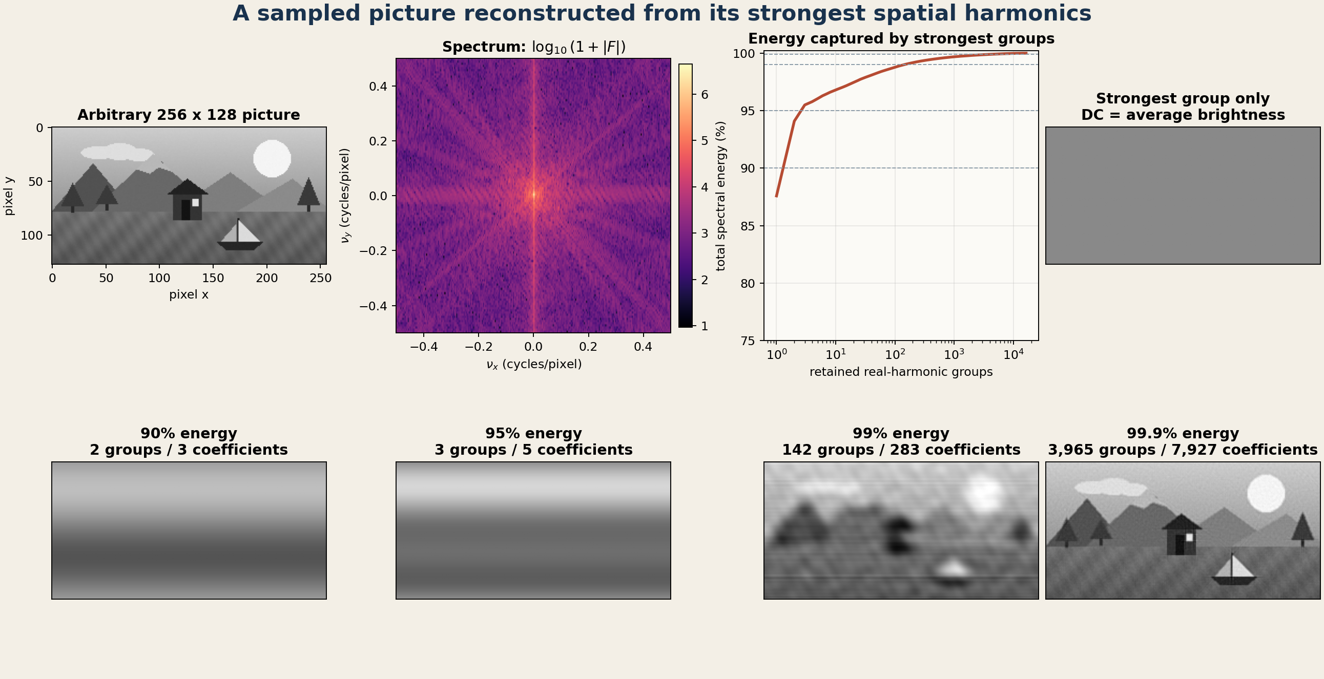
Worked decomposition of textbook Figure 4.0-2. The upper row shows the sampled picture, centered log-magnitude spectrum, cumulative energy, and the DC component alone. The lower row reconstructs the picture after retaining the strongest conjugate-paired real harmonics. Low-frequency terms establish average brightness and broad gradients; many weaker high-frequency terms restore edges and fine texture.

Exact count

The DFT array contains exactly

(3)\[N_{\mathrm{complex}}=N_xN_y=256(128)=\boxed{32{,}768}\]

complex coefficients. For this generated picture, all 32,768 coefficients are nonzero above a numerical tolerance of \(10^{-12}\) times the largest coefficient. Exact zeros are possible for specially symmetric pictures, but the DFT still has 32,768 available harmonic slots and exact reconstruction uses the complete array.

Because the picture is real valued, \(F[-p,-q]=F^*[p,q]\). Most complex exponentials therefore occur in conjugate pairs that combine into one real cosine with an amplitude and a phase. Since both dimensions are even, four bins are self-conjugate: the DC bin and the three combinations of horizontal and vertical Nyquist frequency. The independent real-harmonic group count is consequently

(4)\[N_{\mathrm{real\ groups}} =\frac{32{,}768-4}{2}+4 =\boxed{16{,}386}.\]

The two boxed numbers answer different conventions:

• 32,768 complex spatial harmonics is the direct answer in the complex exponential language used by textbook Figure 4.0-2.

• 16,386 real-harmonic groups is the same information after conjugate partners are combined into real cosines.

For an RGB picture of the same size treated as three separate channels, the direct count would be \(3(32{,}768)=98{,}304\) complex channel coefficients. The pixel pitch is not specified here, so frequencies are in cycles/pixel. For physical pitches \(\Delta x\) and \(\Delta y\), a signed DFT bin \((\widetilde q,\widetilde p)\) represents \(\nu_x=\widetilde q/(N_x\Delta x)\) and \(\nu_y=\widetilde p/(N_y\Delta y)\).

How many are needed for a recognizable picture?

There is no unique number until an error or retained-energy criterion is chosen. Parseval’s theorem makes the coefficient energy \(|F[p,q]|^2\). Sorting conjugate pairs by their combined energy gives the following minimum counts for this particular picture:

Minimum harmonic counts at selected energy thresholds

Energy target	Total-intensity groups	Complex coefficients	Contrast-only groups	Contrast coefficients
90%	2	3	96	192
95%	3	5	324	648
99%	142	283	3,225	6,448
99.9%	3,965	7,927	10,785	21,568

The total-intensity columns include DC. The contrast columns first subtract the mean brightness and measure only non-DC energy; add the one DC group when forming a normally illuminated reconstruction. This is why “90% energy” can be misleading: DC and a broad vertical gradient contain much of the raw numerical energy even though they do not yet make the scene recognizable. The 99% and 99.9% reconstructions show the more useful practical progression.

What do individual components look like?

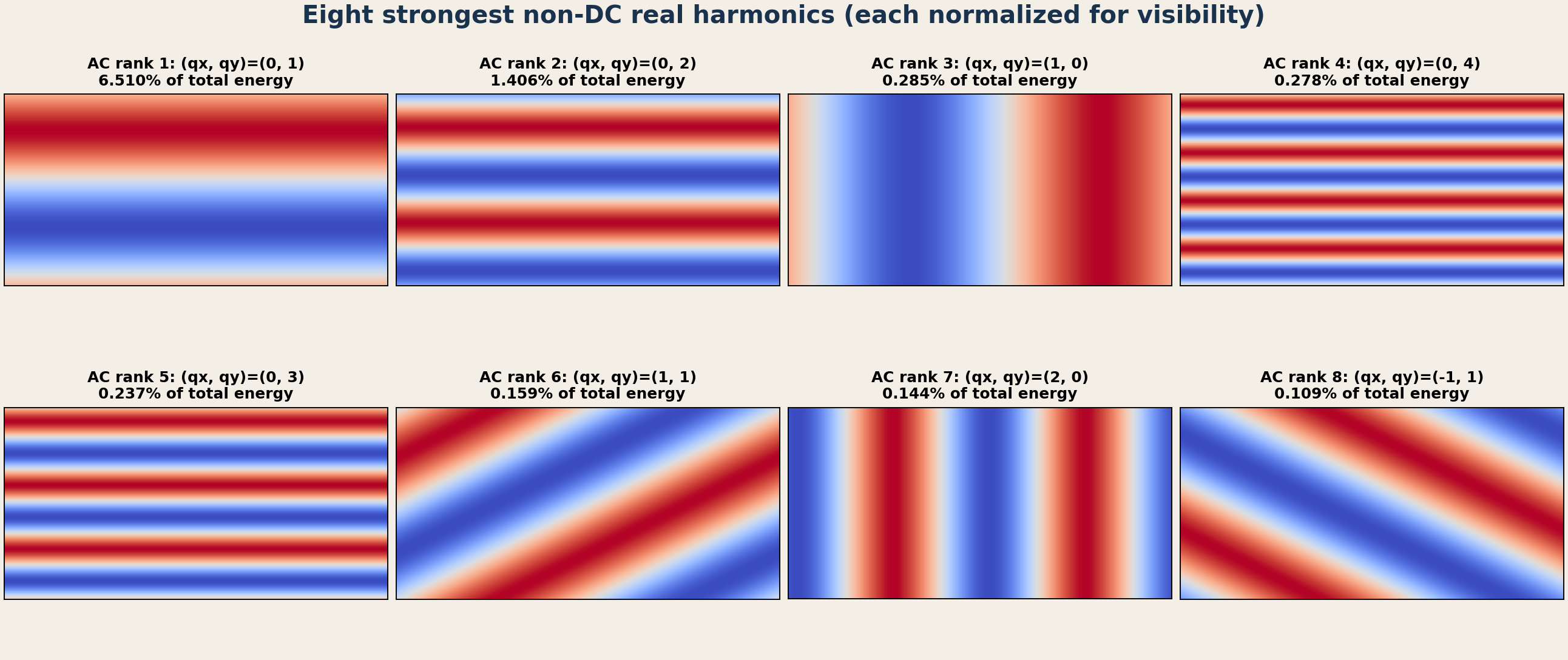
Eight strongest non-DC real harmonics. Each panel is one conjugate pair reconstructed by itself. It is independently normalized so that its stripe orientation and period remain visible; the percentages in the titles, not the displayed color scale, give their true relative energy. Vertical variation in the scene produces horizontal stripes, horizontal variation produces vertical stripes, and simultaneous \(x\) and \(y\) variation produces diagonal stripes.

The complete picture is not stored inside any one component. Every harmonic extends across the whole image; localized mountains, trees, the house, and the boat emerge only after many different amplitudes and phases are added. The figures and counts are reproducible with docs/generate_fourier_picture_decomposition.py.

Section 4.4: why the aperture advice reverses

Two sentences in Sec. 4.4 appear to give opposite advice:

• Sec. 4.4A says that image quality may be improved with a small aperture.

• Example 4.4-1 in Sec. 4.4C says that a smaller F-number, and therefore a larger aperture, gives better image quality.

They do not describe the same limit. Section A studies geometrical blur when the system is not in focus. Section C studies diffraction blur after the system has been set exactly in focus.

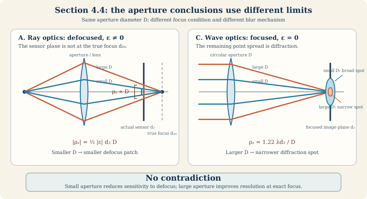
Why the aperture conclusions reverse. On the left, the sensor is displaced from the true image plane, so a wider ray cone makes a wider geometrical patch. On the right, the system is focused and the finite aperture produces diffraction; a wider aperture makes the diffraction spot narrower. The colors identify the aperture cases, not two different wavelengths.

What Sec. 4.4A holds fixed: nonzero focusing error

The section first says that a focused system is ideal within ray theory: each object point maps to one image point. It then changes the condition with the sentence “Suppose now that the system is not in focus” and defines, in textbook Eq. (4.4-1),

(5)\[\epsilon=\frac{1}{d_1}+\frac{1}{d_2}-\frac{1}{f}.\]

Here \(d_2\) is the actual lens-to-image-plane distance. The correctly focused plane would instead be at \(d_{20}\), where \(1/d_1+1/d_{20}=1/f\). A ray passing through the aperture at radius \(\rho\) reaches the actual image plane at blur radius \(\rho_s\). The similar-triangle calculation printed immediately below Fig. 4.4-2 gives

(6)\[\frac{\rho_s}{\rho} =\frac{d_{20}-d_2}{d_{20}} =\epsilon d_2.\]

For a circular aperture, the edge ray has \(\rho=D/2\). Textbook Eq. (4.4-3) is therefore

(7)\[\rho_{s,\mathrm{ray}}=\frac{1}{2}\epsilon d_2D, \qquad |\rho_{s,\mathrm{ray}}| =\frac{1}{2}|\epsilon|d_2D.\]

The second form makes explicit that a physical radius is nonnegative; the sign of \(\epsilon\) identifies which side of focus contains the image plane. With \(\epsilon\ne0\) and \(d_2\) held fixed,

(8)\[|\rho_{s,\mathrm{ray}}|\propto D.\]

Halving \(D\) halves this geometrical defocus patch. This is the precise reason Sec. 4.4A associates a small aperture with reduced sensitivity to focusing error and increased depth of focus. If \(\epsilon=0\), however, Eq. (7) gives zero ray-optics blur for every aperture diameter. The ray model then has nothing more to say about the spot size.

What Example 4.4-1 holds fixed: exact focus

Section 4.4C first defines the generalized pupil in textbook Eq. (4.4-10):

(9)\[p_1(x,y)=p(x,y) \exp\!\left[-j\pi\epsilon\frac{x^2+y^2}{\lambda}\right].\]

Immediately before Example 4.4-1, the book explicitly sets \(\epsilon=0\); hence \(p_1=p\). The example title also specifies a “Focused Imaging System.” The geometrical defocus term has therefore been removed before the circular-aperture result is calculated.

For a circular pupil of diameter \(D\), textbook Eq. (4.4-13) gives the focused amplitude impulse response

(10)\[h(x,y)=h(0,0) \frac{2J_1(\pi D\rho/\lambda d_2)} {\pi D\rho/\lambda d_2}, \qquad \rho=\sqrt{x^2+y^2}.\]

Its first zero occurs at the radius in textbook Eq. (4.4-14),

(11)\[\rho_{s,\mathrm{wave}}=1.22\frac{\lambda d_2}{D}.\]

For focus at infinity, \(d_1=\infty\) and \(d_2=f\), so textbook Eq. (4.4-15) becomes

(12)\[\rho_{s,\mathrm{wave}} =1.22\lambda\frac{f}{D} =1.22\lambda F\#, \qquad F\#=\frac{f}{D}.\]

With \(\lambda\) and \(d_2\) fixed,

(13)\[\rho_{s,\mathrm{wave}}\propto\frac{1}{D}.\]

Halving \(D\) now doubles the diffraction spot. This is why the focused wave-optics example favors a larger aperture. The book immediately qualifies this conclusion by requiring that the larger lens not introduce geometrical aberrations.

Exact comparison

What changes between the two textbook conclusions

Question	Sec. 4.4A	Sec. 4.4C, Example 4.4-1	Aperture advice
Focus condition	Defocused, \(\epsilon\ne0\)	Focused, \(\epsilon=0\)	Different conditions
Optical description	Ray optics	Wave optics	Different models
Source of finite spot	Aperture shadow at the wrong image plane	Diffraction of a circular pupil at the correct image plane	Different mechanisms
Radius scaling	\(|\rho_s|\propto D\)	\(\rho_s\propto1/D\)	Small versus large
What improves	Tolerance to focusing error; depth of focus	Focused resolving power when geometrical aberrations remain negligible	Different performance limits

Important

The exact distinction is not merely “ray optics versus wave optics.” It is also \(\epsilon\ne0\) versus \(\epsilon=0\), meaning an incorrectly located image plane versus the correctly focused plane. The aperture diameter \(D\) is the same kind of quantity in both formulas, but the finite spot has a different cause.

When both finite aperture and defocus are present, Sec. 4.4C points back to the generalized pupil (9): the pupil boundary supplies diffraction while its quadratic phase contains the focusing error. Therefore, the two limiting sentences alone do not imply a universal best aperture and their two spot radii should not simply be added. The generalized pupil must be propagated for the specified \(D\), \(\epsilon\), \(\lambda\), and \(d_2\).

In-text exercises

Exercise 4.1-1 — Binary Fresnel plate

Brief solution

1. Method. The working uses Fourier-transform and convolution identities, exponential, logarithmic, and phasor identities, and algebraic rearrangement and dimensional checks.

2. Reasoning and answer.

\[\boxed{\infty,\ \pm f,\ \pm f/2,\ldots}\]

Show detailed stepsHide detailed steps

Step 1 — Definitions and setup. Symbols are local to this item and follow the chapter convention. Each physical quantity and supplied numerical value is introduced at its first use below; angles are in radians unless a degree symbol is shown, and units are retained through numerical substitution.

Figure 40 — Exercise 4.1-1: Binary Fresnel plate. The diagram identifies the input quantities, physical operation, requested result, variable meanings, and an independent verification route. Every symbol in the variable strip is labeled on the model itself.

Step 2 — Mathematical formulas used. The working uses Fourier-transform and convolution identities, exponential, logarithmic, and phasor identities, and algebraic rearrangement and dimensional checks.

Step 3 — Worked derivation. The calculation is kept in symbolic form until the governing relation has been rearranged for the requested quantity.

Detailed step 1. Expand the binary radial phase in a Fourier series of its quadratic-phase coordinate.

Detailed step 2. Its constant term is an unfocused order; harmonics \(e^{-jqk x^2/(2f)}\) are cylindrical-lens phases.

Detailed step 3. Thus the orders focus at \(\boxed{\infty,\ \pm f,\ \pm f/2,\ldots}\);

Detailed step 4. Fourier coefficients set their amplitudes.

Step 4 — State the numbered result. The principal result obtained in the working is

(14)\[\boxed{\infty,\ \pm f,\ \pm f/2,\ldots}\]

Step 5 — Check. Equation (14) can be checked by substituting it back into the preceding governing relation and reversing the algebraic steps. Transform dimensions and the expected even/odd or conjugate symmetry provide an independent check on signs and scale factors.

Exercise 4.1-2 — Gaussian propagation

Brief solution

1. Method. The working uses Fourier-transform and convolution identities, integration identities, and exponential, logarithmic, and phasor identities.

2. Reasoning and answer.

\[q=z+j\pi W_0^2/\lambda\]

Show detailed stepsHide detailed steps

Step 1 — Definitions and setup. Symbols are local to this item and follow the chapter convention. Each physical quantity and supplied numerical value is introduced at its first use below; angles are in radians unless a degree symbol is shown, and units are retained through numerical substitution.

Figure 41 — Exercise 4.1-2: Gaussian propagation. The diagram identifies the input quantities, physical operation, requested result, variable meanings, and an independent verification route. Every symbol in the variable strip is labeled on the model itself.

Step 2 — Mathematical formulas used. The working uses Fourier-transform and convolution identities, integration identities, and exponential, logarithmic, and phasor identities.

Step 3 — Worked derivation. The calculation is kept in symbolic form until the governing relation has been rearranged for the requested quantity.

Detailed step 1. Fourier transforming \(e^{-\rho^2/W_0^2}\),

Detailed step 2. multiplying by the paraxial free-space transfer function,

Detailed step 3. and transforming back gives \(U=A_0(q_0/q)e^{-jkz}e^{-jk\rho^2/(2q)}\) with \(q=z+j\pi W_0^2/\lambda\).

Detailed step 4. Convolution with the Fresnel kernel gives the same Gaussian integral and therefore the Chapter 3 beam.

Step 4 — State the numbered result. The principal result obtained in the working is

(15)\[q=z+j\pi W_0^2/\lambda\]

Step 5 — Check. Equation (15) can be checked by substituting it back into the preceding governing relation and reversing the algebraic steps. Transform dimensions and the expected even/odd or conjugate symmetry provide an independent check on signs and scale factors.

Exercise 4.2-1 — Fresnel versus Fraunhofer range

Brief solution

1. Method. The working uses algebraic rearrangement and dimensional checks.

2. Reasoning and answer.

\[\boxed{d\gg800\ \mathrm m}\]

Show detailed stepsHide detailed steps

Step 1 — Definitions and setup. Symbols are local to this item and follow the chapter convention. Each physical quantity and supplied numerical value is introduced at its first use below; angles are in radians unless a degree symbol is shown, and units are retained through numerical substitution.

Figure 42 — Exercise 4.2-1: Fresnel versus Fraunhofer range. The diagram identifies the input quantities, physical operation, requested result, variable meanings, and an independent verification route. Every symbol in the variable strip is labeled on the model itself.

Step 2 — Mathematical formulas used. The working uses algebraic rearrangement and dimensional checks.

Step 3 — Worked derivation. The calculation is kept in symbolic form until the governing relation has been rearranged for the requested quantity.

Detailed step 1. For \(a=0.02\) m, \(b=0.01\) m,

Detailed step 2. and \(\lambda=0.5\ \mathrm{\mu m}\),

Detailed step 3. the Fresnel equality estimate is \(d=[(a+b)^4/(4\lambda)]^{1/3}=0.740\) m,

Detailed step 4. so use \(\boxed{d\gg0.740\ \mathrm m}\).

Detailed step 5. Fraunhofer requires both \(a^2/(\lambda d)\ll1\) and \(b^2/(\lambda d)\ll1\); the stricter is \(\boxed{d\gg800\ \mathrm m}\).

Step 4 — State the numbered result. The principal result obtained in the working is

(16)\[\boxed{d\gg800\ \mathrm m}\]

Step 5 — Check. Equation (16) can be checked by substituting it back into the preceding governing relation and reversing the algebraic steps. Check that dimensions agree term by term, then test the simplest symmetry or limiting case for the expected sign and scale. Repeat the substitution with unrounded intermediate values and retain the displayed units; the final unit must have the requested dimension.

Exercise 4.2-2 — Inverse transform

Brief solution

1. Method. The working uses Fourier-transform and convolution identities and exponential, logarithmic, and phasor identities.

Show detailed stepsHide detailed steps

Step 1 — Definitions and setup. Symbols are local to this item and follow the chapter convention. Each physical quantity and supplied numerical value is introduced at its first use below; angles are in radians unless a degree symbol is shown, and units are retained through numerical substitution.

Figure 43 — Exercise 4.2-2: Inverse transform. The diagram identifies the input quantities, physical operation, requested result, variable meanings, and an independent verification route. Every symbol in the variable strip is labeled on the model itself.

Step 2 — Mathematical formulas used. The working uses Fourier-transform and convolution identities and exponential, logarithmic, and phasor identities.

Step 3 — Worked derivation. The calculation is kept in symbolic form until the governing relation has been rearranged for the requested quantity.

Detailed step 1. The focal-plane relation samples \(F(\nu_x,\nu_y)\) at \((x,y)/(\lambda f)\).

Detailed step 2. Reversing focal-plane coordinates changes the kernel from \(e^{-j2\pi\boldsymbol\nu\cdot\mathbf r}\) to \(e^{+j2\pi\boldsymbol\nu\cdot\mathbf r}\),

Detailed step 3. which is exactly the inverse Fourier transform.

Step 4 — Interpret the result. The final relation or conclusion in Step 3 is the requested result. Read its sign, scale, or physical classification using the conventions fixed in Step 1.

Step 5 — Check. Transform dimensions and the expected even/odd or conjugate symmetry provide an independent check on signs and scale factors.

Exercise 4.3-1 — Rectangular aperture

Brief solution

1. Method. The working uses Fourier-transform and convolution identities and algebraic rearrangement and dimensional checks.

2. Reasoning and answer.

\[y=\pm\lambda d/D_y\]

Show detailed stepsHide detailed steps

Step 1 — Definitions and setup. Symbols are local to this item and follow the chapter convention. Each physical quantity and supplied numerical value is introduced at its first use below; angles are in radians unless a degree symbol is shown, and units are retained through numerical substitution.

Figure 44 — Exercise 4.3-1: Rectangular aperture. The diagram identifies the input quantities, physical operation, requested result, variable meanings, and an independent verification route. Every symbol in the variable strip is labeled on the model itself.

Step 2 — Mathematical formulas used. The working uses Fourier-transform and convolution identities and algebraic rearrangement and dimensional checks.

Step 3 — Worked derivation. The calculation is kept in symbolic form until the governing relation has been rearranged for the requested quantity.

Detailed step 1. The transform of \(\operatorname{rect}(x/D_x) \operatorname{rect}(y/D_y)\) is \(D_xD_y\operatorname{sinc}(D_x\nu_x) \operatorname{sinc}(D_y\nu_y)\).

Detailed step 2. Squaring at \(\nu_{x,y}=(x,y)/(\lambda d)\) gives Eq. (4.3-6),

Detailed step 3. with first zeros \(x=\pm\lambda d/D_x\), \(y=\pm\lambda d/D_y\).

Step 4 — State the numbered result. The principal result obtained in the working is

(17)\[y=\pm\lambda d/D_y\]

Step 5 — Check. Equation (17) can be checked by substituting it back into the preceding governing relation and reversing the algebraic steps. Transform dimensions and the expected even/odd or conjugate symmetry provide an independent check on signs and scale factors.

Exercise 4.3-2 — Circular aperture

Brief solution

1. Method. The working uses Fourier-transform and convolution identities, integration identities, and algebraic rearrangement and dimensional checks.

2. Reasoning and answer.

\[\boxed{\theta_s=1.22\lambda/D}\]

Show detailed stepsHide detailed steps

Step 1 — Definitions and setup. Symbols are local to this item and follow the chapter convention. Each physical quantity and supplied numerical value is introduced at its first use below; angles are in radians unless a degree symbol is shown, and units are retained through numerical substitution.

Figure 45 — Exercise 4.3-2: Circular aperture. The diagram identifies the input quantities, physical operation, requested result, variable meanings, and an independent verification route. Every symbol in the variable strip is labeled on the model itself.

Step 2 — Mathematical formulas used. The working uses Fourier-transform and convolution identities, integration identities, and algebraic rearrangement and dimensional checks.

Step 3 — Worked derivation. The calculation is kept in symbolic form until the governing relation has been rearranged for the requested quantity.

Detailed step 1. The polar Fourier integral gives \(2J_1(\pi D\rho/\lambda d)/(\pi D\rho/\lambda d)\).

Detailed step 2. Its first numerator zero is 3.8317,

Detailed step 3. hence \(\boxed{\rho_s=1.22\lambda d/D}\) and \(\boxed{\theta_s=1.22\lambda/D}\).

Step 4 — State the numbered result. The principal result obtained in the working is

(18)\[\boxed{\theta_s=1.22\lambda/D}\]

Step 5 — Check. Equation (18) can be checked by substituting it back into the preceding governing relation and reversing the algebraic steps. Transform dimensions and the expected even/odd or conjugate symmetry provide an independent check on signs and scale factors.

Exercise 4.3-3 — Focused spot

Brief solution

1. Method. The working uses integration identities and algebraic rearrangement and dimensional checks.

Show detailed stepsHide detailed steps

Step 1 — Definitions and setup. Symbols are local to this item and follow the chapter convention. Each physical quantity and supplied numerical value is introduced at its first use below; angles are in radians unless a degree symbol is shown, and units are retained through numerical substitution.

Figure 46 — Exercise 4.3-3: Focused spot. The diagram identifies the input quantities, physical operation, requested result, variable meanings, and an independent verification route. Every symbol in the variable strip is labeled on the model itself.

Step 2 — Mathematical formulas used. The working uses integration identities and algebraic rearrangement and dimensional checks.

Step 3 — Worked derivation. The calculation is kept in symbolic form until the governing relation has been rearranged for the requested quantity.

Detailed step 1. Replace propagation distance by focal length in the preceding result: \(\rho_s=1.22\lambda f/D\).

Detailed step 2. A Gaussian filling a clear diameter near \(D\simeq2W\) has \(W'_0=\lambda f/(\pi W)\simeq0.637\lambda f/D\); the differing radius definitions explain the numerical factor.

End-of-chapter problems

Step 4 — State the numbered result. The principal result obtained in the working is

(19)\[W'_0=\lambda f/(\pi W)\simeq0.637\lambda f/D\]

Step 5 — Check. Equation (19) can be checked by substituting it back into the preceding governing relation and reversing the algebraic steps. Differentiation of an antiderivative, or normalization of a definite integral, checks the integration step. Repeat the substitution with unrounded intermediate values and retain the displayed units; the final unit must have the requested dimension.

Problem 4.1-3 — Harmonic propagation

Brief solution

1. Method. The working uses exponential, logarithmic, and phasor identities and algebraic rearrangement and dimensional checks.

2. Reasoning and answer.

\[\nu_x=m/(20\lambda)\]

Show detailed stepsHide detailed steps

Definitions and setup. Symbols are local to this item and follow the chapter convention. Each physical quantity and supplied numerical value is introduced at its first use below; angles are in radians unless a degree symbol is shown, and units are retained through numerical substitution.

Mathematical formulas used. The working uses exponential, logarithmic, and phasor identities and algebraic rearrangement and dimensional checks.

Worked derivation. The calculation is kept in symbolic form until the governing relation has been rearranged for the requested quantity.

Detailed step 1. Decompose each input into terms \(c_m e^{j2\pi(\nu_{xm}x+\nu_{ym}y)}\) and multiply by \(H_m=e^{-j2\pi d\sqrt{\lambda^{-2}-\nu_{xm}^2-\nu_{ym}^2}}\).

Detailed step 2. This leaves (a) one axial plane wave; (b) one oblique wave with \((\nu_x,\nu_y)=(-1/2\lambda,-1/2\lambda)\); (c) two waves at \(\nu_x=\pm1/(4\lambda)\); (d) an axial term plus two at \(\nu_y=\pm1/(2\lambda)\); and (e) grating orders \(\nu_x=m/(20\lambda)\) weighted by the 50%-duty rectangular-cell coefficients.

Numbered result. The principal result obtained in the working is

(20)\[\nu_x=m/(20\lambda)\]

Check. Equation (20) can be checked by substituting it back into the preceding governing relation and reversing the algebraic steps. Check that dimensions agree term by term, then test the simplest symmetry or limiting case for the expected sign and scale.

Problem 4.1-4 — Direction cone

Brief solution

1. Method. The working uses trigonometric and small-angle identities and algebraic rearrangement and dimensional checks.

2. Reasoning and answer.

\[\boxed{\theta_{max}=7.27^\circ}\]

Show detailed stepsHide detailed steps

Definitions and setup. Symbols are local to this item and follow the chapter convention. Each physical quantity and supplied numerical value is introduced at its first use below; angles are in radians unless a degree symbol is shown, and units are retained through numerical substitution.

Mathematical formulas used. The working uses trigonometric and small-angle identities and algebraic rearrangement and dimensional checks.

Worked derivation. The calculation is kept in symbolic form until the governing relation has been rearranged for the requested quantity.

Detailed step 1. \(\sin\theta_{max}=\lambda\nu_{max}=(0.000633)(200)=0.1266\),

Detailed step 2. so \(\boxed{\theta_{max}=7.27^\circ}\).

Numbered result. The principal result obtained in the working is

(21)\[\boxed{\theta_{max}=7.27^\circ}\]

Check. Equation (21) can be checked by substituting it back into the preceding governing relation and reversing the algebraic steps. The zero-angle or paraxial limit supplies an independent sign and magnitude check whenever that limit is part of the model. Repeat the substitution with unrounded intermediate values and retain the displayed units; the final unit must have the requested dimension.

Problem 4.1-5 — Logarithmic map

Brief solution

1. Method. The working uses product, quotient, and chain rules, integration identities, and exponential, logarithmic, and phasor identities.

2. Reasoning and answer.

\[\boxed{\phi=-(x\ln x-x)/(\lambda f)+C}\]

Show detailed stepsHide detailed steps

Definitions and setup. Symbols are local to this item and follow the chapter convention. Each physical quantity and supplied numerical value is introduced at its first use below; angles are in radians unless a degree symbol is shown, and units are retained through numerical substitution.

Mathematical formulas used. The working uses product, quotient, and chain rules, integration identities, and exponential, logarithmic, and phasor identities.

Worked derivation. The calculation is kept in symbolic form until the governing relation has been rearranged for the requested quantity.

Detailed step 1. A phase \(t=e^{-j2\pi\phi}\) deflects by \(\theta=-\lambda\phi'\).

Detailed step 2. With a lens, \(\phi'=-(\ln x)/(\lambda f)\),

Detailed step 3. hence \(\boxed{\phi=-(x\ln x-x)/(\lambda f)+C}\).

Detailed step 4. If light instead propagates distance \(f\) without the lens,

Detailed step 5. require \(x+f\theta=\ln x\); replace the derivative by \(\phi'=-(\ln x-x)/(\lambda f)\) and integrate.

Numbered result. The principal result obtained in the working is

(22)\[\boxed{\phi=-(x\ln x-x)/(\lambda f)+C}\]

Check. Equation (22) can be checked by substituting it back into the preceding governing relation and reversing the algebraic steps. Differentiation of an antiderivative, or normalization of a definite integral, checks the integration step.

Problem 4.2-3 — Lens Fourier-transform proof

Brief solution

1. Method. The working uses Fourier-transform and convolution identities, exponential, logarithmic, and phasor identities, and algebraic rearrangement and dimensional checks.

2. Reasoning and answer.

\[g(x)=e^{-j2kf}F[x/(\lambda f)]/(j\lambda f)\]

Show detailed stepsHide detailed steps

Definitions and setup. Symbols are local to this item and follow the chapter convention. Each physical quantity and supplied numerical value is introduced at its first use below; angles are in radians unless a degree symbol is shown, and units are retained through numerical substitution.

Mathematical formulas used. The working uses Fourier-transform and convolution identities, exponential, logarithmic, and phasor identities, and algebraic rearrangement and dimensional checks.

Worked derivation. The calculation is kept in symbolic form until the governing relation has been rearranged for the requested quantity.

Detailed step 1. Expand \((x-x')^2=x^2+x'^2-2xx'\) in the Fresnel convolution.

Detailed step 2. The two quadratic factors surround the Fourier kernel.

Detailed step 3. In the propagation–lens– propagation cascade the lens cancels both inner quadratic phases,

Detailed step 4. leaving \(g(x)=e^{-j2kf}F[x/(\lambda f)]/(j\lambda f)\) up to convention phase.

Numbered result. The principal result obtained in the working is

(23)\[g(x)=e^{-j2kf}F[x/(\lambda f)]/(j\lambda f)\]

Check. Equation (23) can be checked by substituting it back into the preceding governing relation and reversing the algebraic steps. Transform dimensions and the expected even/odd or conjugate symmetry provide an independent check on signs and scale factors.

Problem 4.2-4 — Line-function transforms

Brief solution

1. Method. The working uses Fourier-transform and convolution identities, exponential, logarithmic, and phasor identities, and trigonometric and small-angle identities.

2. Reasoning and answer.

\[\lambda f=1\ \mathrm{mm^2}\]

Show detailed stepsHide detailed steps

Definitions and setup. Symbols are local to this item and follow the chapter convention. Each physical quantity and supplied numerical value is introduced at its first use below; angles are in radians unless a degree symbol is shown, and units are retained through numerical substitution.

Mathematical formulas used. The working uses Fourier-transform and convolution identities, exponential, logarithmic, and phasor identities, and trigonometric and small-angle identities.

Worked derivation. The calculation is kept in symbolic form until the governing relation has been rearranged for the requested quantity.

Detailed step 1. (a) \(\delta(x-y)\) is a bright diagonal in both planes,

Detailed step 2. rotated to its orthogonal Fourier line. (b) Two lines at \(x=\pm a\) transform to \(2\cos(2\pi a\nu_x)\),

Detailed step 3. giving cosine-squared fringes. (c) Relative phase \(j\) changes this to \(e^{j2\pi a\nu_x}+j e^{-j2\pi a\nu_x}\) and shifts the fringes by one quarter period.

Detailed step 4. Use \(x_f=\lambda f\nu_x\); here \(\lambda f=1\ \mathrm{mm^2}\).

Numbered result. The principal result obtained in the working is

(24)\[\lambda f=1\ \mathrm{mm^2}\]

Check. Equation (24) can be checked by substituting it back into the preceding governing relation and reversing the algebraic steps. Transform dimensions and the expected even/odd or conjugate symmetry provide an independent check on signs and scale factors. Repeat the substitution with unrounded intermediate values and retain the displayed units; the final unit must have the requested dimension.

Problem 4.2-5 — Fourier-plane scale

Brief solution

1. Method. The working uses Fourier-transform and convolution identities and algebraic rearrangement and dimensional checks.

2. Reasoning and answer.

\[\boxed{f=0.09/[488\times10^{-9}(180\times10^3)] =1.025\ \mathrm m}\]

Show detailed stepsHide detailed steps

Definitions and setup. Symbols are local to this item and follow the chapter convention. Each physical quantity and supplied numerical value is introduced at its first use below; angles are in radians unless a degree symbol is shown, and units are retained through numerical substitution.

Mathematical formulas used. The working uses Fourier-transform and convolution identities and algebraic rearrangement and dimensional checks.

Worked derivation. The calculation is kept in symbolic form until the governing relation has been rearranged for the requested quantity.

Detailed step 1. \(\Delta x=\lambda f(200-20)\) lines/mm.

Detailed step 2. Therefore \(\boxed{f=0.09/[488\times10^{-9}(180\times10^3)] =1.025\ \mathrm m}\).

Numbered result. The principal result obtained in the working is

(25)\[\boxed{f=0.09/[488\times10^{-9}(180\times10^3)] =1.025\ \mathrm m}\]

Check. Equation (25) can be checked by substituting it back into the preceding governing relation and reversing the algebraic steps. Transform dimensions and the expected even/odd or conjugate symmetry provide an independent check on signs and scale factors. Repeat the substitution with unrounded intermediate values and retain the displayed units; the final unit must have the requested dimension.

Problem 4.3-4 — Multi-slit grating

Brief solution

1. Method. The working uses exponential, logarithmic, and phasor identities, trigonometric and small-angle identities, and algebraic rearrangement and dimensional checks.

2. Key step.

The field is \(\sum_{m=-L}^{L}e^{-j2\pi ma\theta/\lambda}\) and the intensity is

3. Answer.

\[\boxed{I\propto\left[ \frac{\sin(M\pi a\theta/\lambda)} {\sin(\pi a\theta/\lambda)}\right]^2}.\]

Principal orders occur at \(\theta_q\simeq q\lambda/a=q/10\); adjacent zeros are \(1/M\) of that separation away.

Show detailed stepsHide detailed steps

Definitions and setup. Symbols are local to this item and follow the chapter convention. Each physical quantity and supplied numerical value is introduced at its first use below; angles are in radians unless a degree symbol is shown, and units are retained through numerical substitution.

Mathematical formulas used. The working uses exponential, logarithmic, and phasor identities, trigonometric and small-angle identities, and algebraic rearrangement and dimensional checks.

Worked derivation. The calculation is kept in symbolic form until the governing relation has been rearranged for the requested quantity.

The field is \(\sum_{m=-L}^{L}e^{-j2\pi ma\theta/\lambda}\) and the intensity is

(26)\[\boxed{I\propto\left[ \frac{\sin(M\pi a\theta/\lambda)} {\sin(\pi a\theta/\lambda)}\right]^2}.\]

Principal orders occur at \(\theta_q\simeq q\lambda/a=q/10\); adjacent zeros are \(1/M\) of that separation away.

Check. Equation (26) can be checked by substituting it back into the preceding governing relation and reversing the algebraic steps. The zero-angle or paraxial limit supplies an independent sign and magnitude check whenever that limit is part of the model.

Problem 4.3-5 — Oblique Fraunhofer illumination

Brief solution

1. Method. The working uses exponential, logarithmic, and phasor identities and algebraic rearrangement and dimensional checks.

2. Reasoning and answer.

\[\boxed{I(x,y)\propto|P(x/\lambda d-\nu_{0x},y/\lambda d)|^2}\]

Show detailed stepsHide detailed steps

Definitions and setup. Symbols are local to this item and follow the chapter convention. Each physical quantity and supplied numerical value is introduced at its first use below; angles are in radians unless a degree symbol is shown, and units are retained through numerical substitution.

Mathematical formulas used. The working uses exponential, logarithmic, and phasor identities and algebraic rearrangement and dimensional checks.

Worked derivation. The calculation is kept in symbolic form until the governing relation has been rearranged for the requested quantity.

Detailed step 1. The aperture field gains \(e^{-j2\pi\nu_{0x}x}\) with \(\nu_{0x}\simeq\theta_x/\lambda\).

Detailed step 2. The shift theorem gives \(\boxed{I(x,y)\propto|P(x/\lambda d-\nu_{0x},y/\lambda d)|^2}\): the entire pattern shifts by \(d\theta_x\).

Numbered result. The principal result obtained in the working is

(27)\[\boxed{I(x,y)\propto|P(x/\lambda d-\nu_{0x},y/\lambda d)|^2}\]

Check. Equation (27) can be checked by substituting it back into the preceding governing relation and reversing the algebraic steps. Check that dimensions agree term by term, then test the simplest symmetry or limiting case for the expected sign and scale.

Problem 4.3-6 — Two-pinhole Fresnel pattern

Brief solution

1. Method. The working uses trigonometric and small-angle identities and algebraic rearrangement and dimensional checks.

2. Reasoning and answer.

\[\boxed{I=(2/\lambda d)^2\cos^2(2\pi ax/\lambda d)}\]

Show detailed stepsHide detailed steps

Definitions and setup. Symbols are local to this item and follow the chapter convention. Each physical quantity and supplied numerical value is introduced at its first use below; angles are in radians unless a degree symbol is shown, and units are retained through numerical substitution.

Mathematical formulas used. The working uses trigonometric and small-angle identities and algebraic rearrangement and dimensional checks.

Worked derivation. The calculation is kept in symbolic form until the governing relation has been rearranged for the requested quantity.

Detailed step 1. Adding the two Fresnel kernels cancels their common phase and leaves \(2\cos(2\pi ax/\lambda d)\).

Detailed step 2. Squaring gives \(\boxed{I=(2/\lambda d)^2\cos^2(2\pi ax/\lambda d)}\).

Numbered result. The principal result obtained in the working is

(28)\[\boxed{I=(2/\lambda d)^2\cos^2(2\pi ax/\lambda d)}\]

Check. Equation (28) can be checked by substituting it back into the preceding governing relation and reversing the algebraic steps. The zero-angle or paraxial limit supplies an independent sign and magnitude check whenever that limit is part of the model.

Problem 4.3-7 — Fresnel/Fraunhofer relation

Brief solution

1. Method. The working uses Fourier-transform and convolution identities, integration identities, and exponential, logarithmic, and phasor identities.

Show detailed stepsHide detailed steps

Definitions and setup. Symbols are local to this item and follow the chapter convention. Each physical quantity and supplied numerical value is introduced at its first use below; angles are in radians unless a degree symbol is shown, and units are retained through numerical substitution.

Mathematical formulas used. The working uses Fourier-transform and convolution identities, integration identities, and exponential, logarithmic, and phasor identities.

Worked derivation. The calculation is kept in symbolic form until the governing relation has been rearranged for the requested quantity.

Detailed step 1. Expanding the Fresnel kernel shows that its integral is the Fourier transform of \(p(x',y')e^{-j\pi(x'^2+y'^2)/(\lambda d)}\) evaluated at \((x,y)/(\lambda d)\),

Detailed step 2. times an output quadratic phase.

Detailed step 3. Its magnitude is therefore the requested Fraunhofer pattern.

Check. Transform dimensions and the expected even/odd or conjugate symmetry provide an independent check on signs and scale factors.

Problem 4.4-1 — Blurred sinusoidal grating

Brief solution

1. Method. The working uses trigonometric and small-angle identities and algebraic rearrangement and dimensional checks.

2. Reasoning and answer.

\[\boxed{C=|\operatorname{sinc}(2D/a)|}\]

Show detailed stepsHide detailed steps

Definitions and setup. Symbols are local to this item and follow the chapter convention. Each physical quantity and supplied numerical value is introduced at its first use below; angles are in radians unless a degree symbol is shown, and units are retained through numerical substitution.

Mathematical formulas used. The working uses trigonometric and small-angle identities and algebraic rearrangement and dimensional checks.

Worked derivation. The calculation is kept in symbolic form until the governing relation has been rearranged for the requested quantity.

Detailed step 1. Convolving \([1+\cos(4\pi x/a)]/2\) with a width-\(D\) square gives \(g(x,0)=D[1+\operatorname{sinc}(2D/a)\cos(4\pi x/a)]/2\) (apart from the constant y factor).

Detailed step 2. Thus \(\boxed{C=|\operatorname{sinc}(2D/a)|}\).

Numbered result. The principal result obtained in the working is

(29)\[\boxed{C=|\operatorname{sinc}(2D/a)|}\]

Check. Equation (29) can be checked by substituting it back into the preceding governing relation and reversing the algebraic steps. The zero-angle or paraxial limit supplies an independent sign and magnitude check whenever that limit is part of the model.

Problem 4.4-2 — Phase-edge image

Brief solution

1. Method. The working uses integration identities, exponential, logarithmic, and phasor identities, and algebraic rearrangement and dimensional checks.

2. Reasoning and answer.

\[x=0\]

Show detailed stepsHide detailed steps

Definitions and setup. Symbols are local to this item and follow the chapter convention. Each physical quantity and supplied numerical value is introduced at its first use below; angles are in radians unless a degree symbol is shown, and units are retained through numerical substitution.

Mathematical formulas used. The working uses integration identities, exponential, logarithmic, and phasor identities, and algebraic rearrangement and dimensional checks.

Worked derivation. The calculation is kept in symbolic form until the governing relation has been rearranged for the requested quantity.

Detailed step 1. Because \(h=\operatorname{rect}(x)\delta(y)\),

Detailed step 2. the output is the running unit-width average \(g(x,y)=\int_{x-1/2}^{x+1/2}f(u,y)du\).

Detailed step 3. Far from the phase edge its magnitude is one; while the window straddles \(x=0\),

Detailed step 4. the two constant phasors add in proportions \(1/2\pm x\).

Detailed step 5. Squaring this piecewise linear phasor gives the nonuniform transition intensity.

Numbered result. The principal result obtained in the working is

(30)\[x=0\]

Check. Equation (30) can be checked by substituting it back into the preceding governing relation and reversing the algebraic steps. Differentiation of an antiderivative, or normalization of a definite integral, checks the integration step.

Problem 4.4-3 — Spatial filtering

Brief solution

1. Method. The working uses Fourier-transform and convolution identities, vector-calculus identities, and algebraic rearrangement and dimensional checks.

2. Reasoning and answer.

\[\boxed{p(x_f,y_f)=-4\pi^2(x_f^2+y_f^2)/(\lambda f)^2}\]

Show detailed stepsHide detailed steps

Definitions and setup. Symbols are local to this item and follow the chapter convention. Each physical quantity and supplied numerical value is introduced at its first use below; angles are in radians unless a degree symbol is shown, and units are retained through numerical substitution.

Mathematical formulas used. The working uses Fourier-transform and convolution identities, vector-calculus identities, and algebraic rearrangement and dimensional checks.

Worked derivation. The calculation is kept in symbolic form until the governing relation has been rearranged for the requested quantity.

Detailed step 1. With \(\lambda f=1\ \mathrm{mm^2}\), \(g=\mathcal F^{-1}\{F(\nu)p(\nu)\}\).

Detailed step 2. Hence (a) \(g(x,0)=\operatorname{sinc}(x-5)\); (b) \(g(x,0)=\operatorname{tri}(x)\).

Detailed step 3. A Laplacian filter uses \(\boxed{p(x_f,y_f)=-4\pi^2(x_f^2+y_f^2)/(\lambda f)^2}\) within the available pupil.

Numbered result. The principal result obtained in the working is

(31)\[\boxed{p(x_f,y_f)=-4\pi^2(x_f^2+y_f^2)/(\lambda f)^2}\]

Check. Equation (31) can be checked by substituting it back into the preceding governing relation and reversing the algebraic steps. Transform dimensions and the expected even/odd or conjugate symmetry provide an independent check on signs and scale factors. Repeat the substitution with unrounded intermediate values and retain the displayed units; the final unit must have the requested dimension.

Problem 4.4-4 — Optical cross-correlation

Brief solution

1. Method. The working uses Fourier-transform and convolution identities.

Show detailed stepsHide detailed steps

Definitions and setup. Symbols are local to this item and follow the chapter convention. Each physical quantity and supplied numerical value is introduced at its first use below; angles are in radians unless a degree symbol is shown, and units are retained through numerical substitution.

Mathematical formulas used. The working uses Fourier-transform and convolution identities.

Worked derivation. The calculation is kept in symbolic form until the governing relation has been rearranged for the requested quantity.

Detailed step 1. Place \(f_1\) at the input and \(F_2^*(\nu_x,\nu_y)\) in the Fourier plane.

Detailed step 2. The inverse-transform plane then contains \(f_1\star f_2\).

Detailed step 3. All masks can be real only when the needed spectra have zero/constant phase (for example,

Detailed step 4. real even functions); a general real image still has a complex Fourier transform.

Check. Transform dimensions and the expected even/odd or conjugate symmetry provide an independent check on signs and scale factors.

Problem 4.4-5 — Severe defocus

Brief solution

1. Method. The working uses stationary-value condition, integration identities, and algebraic rearrangement and dimensional checks.

2. Reasoning and answer.

\[\boxed{h(x,y)\propto p(x/(\epsilon d_2),y/(\epsilon d_2))}\]

Show detailed stepsHide detailed steps

Definitions and setup. Symbols are local to this item and follow the chapter convention. Each physical quantity and supplied numerical value is introduced at its first use below; angles are in radians unless a degree symbol is shown, and units are retained through numerical substitution.

Mathematical formulas used. The working uses stationary-value condition, integration identities, and algebraic rearrangement and dimensional checks.

Worked derivation. The calculation is kept in symbolic form until the governing relation has been rearranged for the requested quantity.

Detailed step 1. In the diffraction integral the rapidly varying phase has stationary point \((x',y')=(x/(\epsilon d_2),y/(\epsilon d_2))\).

Detailed step 2. Stationary-phase evaluation makes all slowly varying factors constant there and gives \(\boxed{h(x,y)\propto p(x/(\epsilon d_2),y/(\epsilon d_2))}\) up to the book’s normalization and phase,

Detailed step 3. the same geometrical pupil image.

Numbered result. The principal result obtained in the working is

(32)\[\boxed{h(x,y)\propto p(x/(\epsilon d_2),y/(\epsilon d_2))}\]

Check. Equation (32) can be checked by substituting it back into the preceding governing relation and reversing the algebraic steps. Differentiation of an antiderivative, or normalization of a definite integral, checks the integration step.

Problem 4.4-6 — Resolving two points

Brief solution

1. Method. The working uses common differential-equation solutions and algebraic rearrangement and dimensional checks.

2. Reasoning and answer.

\[\boxed{b\simeq0.1325\ \mathrm{mm}}\]

Show detailed stepsHide detailed steps

Definitions and setup. Symbols are local to this item and follow the chapter convention. Each physical quantity and supplied numerical value is introduced at its first use below; angles are in radians unless a degree symbol is shown, and units are retained through numerical substitution.

Mathematical formulas used. The working uses common differential-equation solutions and algebraic rearrangement and dimensional checks.

Worked derivation. The calculation is kept in symbolic form until the governing relation has been rearranged for the requested quantity.

Detailed step 1. For a square pupil, \(h\propto\operatorname{sinc}(Dx/\lambda d_2) \operatorname{sinc}(Dy/\lambda d_2)\).

Detailed step 2. Two points give \(g=h(x,y)+h(x-b,y)\).

Detailed step 3. With \(\lambda d_2/D=0.1\) mm,

Detailed step 4. all three listed separations (0.5, 1, 2 mm) show two clear peaks.

Detailed step 5. Solving \(g''(b/2)=0\) gives the equal-phase two-peak threshold \(\boxed{b\simeq0.1325\ \mathrm{mm}}\).

Numbered result. The principal result obtained in the working is

(33)\[\boxed{b\simeq0.1325\ \mathrm{mm}}\]

Check. Equation (33) can be checked by substituting it back into the preceding governing relation and reversing the algebraic steps. Differentiating the proposed solution and substituting it into the original differential equation verifies the functional form. Repeat the substitution with unrounded intermediate values and retain the displayed units; the final unit must have the requested dimension.

Problem 4.4-7 — Annular pupil

Brief solution

1. Method. The working uses algebraic rearrangement and dimensional checks.

2. Reasoning and answer.

\[\boxed{4.375,5.250\ \mathrm{mm}}\]

Show detailed stepsHide detailed steps

Definitions and setup. Symbols are local to this item and follow the chapter convention. Each physical quantity and supplied numerical value is introduced at its first use below; angles are in radians unless a degree symbol is shown, and units are retained through numerical substitution.

Mathematical formulas used. The working uses algebraic rearrangement and dimensional checks.

Worked derivation. The calculation is kept in symbolic form until the governing relation has been rearranged for the requested quantity.

Detailed step 1. At unit magnification \(d_1=d_2=2f=2\) m.

Detailed step 2. The coherent transfer function is an annulus with spatial-frequency radii \(a/(\lambda d_2)=2.5\) and \(b/(\lambda d_2)=3.0\) lines/mm.

Detailed step 3. Moving the image plane to 0.25 m maps the physical pupil by ray scale \(1+d_2(1/d_1-1/f)=0.875\); the impulse response is therefore an annulus of radii \(\boxed{4.375,5.250\ \mathrm{mm}}\) (apart from phase and scale).

Numbered result. The principal result obtained in the working is

(34)\[\boxed{4.375,5.250\ \mathrm{mm}}\]

Check. Equation (34) can be checked by substituting it back into the preceding governing relation and reversing the algebraic steps. Check that dimensions agree term by term, then test the simplest symmetry or limiting case for the expected sign and scale. Repeat the substitution with unrounded intermediate values and retain the displayed units; the final unit must have the requested dimension.

Problem 4.5-1 — Spherical-reference holography

Brief solution

1. Method. The working uses exponential, logarithmic, and phasor identities and algebraic rearrangement and dimensional checks.

2. Reasoning and answer.

\[|O+R|^2=|O|^2+|R|^2+OR^*+O^*R\]

Show detailed stepsHide detailed steps

Definitions and setup. Symbols are local to this item and follow the chapter convention. Each physical quantity and supplied numerical value is introduced at its first use below; angles are in radians unless a degree symbol is shown, and units are retained through numerical substitution.

Mathematical formulas used. The working uses exponential, logarithmic, and phasor identities and algebraic rearrangement and dimensional checks.

Worked derivation. The calculation is kept in symbolic form until the governing relation has been rearranged for the requested quantity.

Detailed step 1. Record \(|O+R|^2=|O|^2+|R|^2+OR^*+O^*R\),

Detailed step 2. using \(R\propto e^{-jk\rho^2/(2d)}\).

Detailed step 3. On replay with \(R\),

Detailed step 4. the \(OR^*\) term reconstructs \(O\); the conjugate term creates the twin image.

Detailed step 5. A tilted plane object makes an off-axis Fresnel-zone pattern; a displaced spherical object makes the difference of two quadratic phases and therefore shifted zone plates whose curvature encodes \(d_1^{-1}-d^{-1}\).

Numbered result. The principal result obtained in the working is

(35)\[|O+R|^2=|O|^2+|R|^2+OR^*+O^*R\]

Check. Equation (35) can be checked by substituting it back into the preceding governing relation and reversing the algebraic steps. Check that dimensions agree term by term, then test the simplest symmetry or limiting case for the expected sign and scale.

Problem 4.5-2 — Joint-transform correlation

Brief solution

1. Method. The working uses Fourier-transform and convolution identities, exponential, logarithmic, and phasor identities, and algebraic rearrangement and dimensional checks.

2. Reasoning and answer.

\[x=\pm2a\]

Show detailed stepsHide detailed steps

Definitions and setup. Symbols are local to this item and follow the chapter convention. Each physical quantity and supplied numerical value is introduced at its first use below; angles are in radians unless a degree symbol is shown, and units are retained through numerical substitution.

Mathematical formulas used. The working uses Fourier-transform and convolution identities, exponential, logarithmic, and phasor identities, and algebraic rearrangement and dimensional checks.

Worked derivation. The calculation is kept in symbolic form until the governing relation has been rearranged for the requested quantity.

Detailed step 1. For separated inputs the recorded spectrum contains \(F_1F_2^*e^{-j4\pi a\nu_x}\) and its conjugate besides the two autocorrelation terms.

Detailed step 2. A second Fourier transform produces separated peaks \(f_1\star f_2\) and \(f_2\star f_1\) at \(x=\pm2a\); reading either off-axis term yields the desired cross-correlation without overlap.

Numbered result. The principal result obtained in the working is

(36)\[x=\pm2a\]

Check. Equation (36) can be checked by substituting it back into the preceding governing relation and reversing the algebraic steps. Transform dimensions and the expected even/odd or conjugate symmetry provide an independent check on signs and scale factors.