Photonics Essentials: From Diffusion Current to Equation 3.5

Source

Thomas P. Pearsall, Photonics Essentials: An Introduction with Experiments (McGraw-Hill, 2003), Chapter 3, Photodiodes, printed pages 38–40.

Question

The chapter first gives a diffusion-current equation containing one spatial derivative,

\[J(x)=-qD_e\frac{\partial n}{\partial x}.\]

Why does the carrier equation later contain the second derivative \(\partial^2 n/\partial x^2\)?

Important

Current \(J\) does not turn directly into concentration. Equation 3.5 asks whether more carriers enter a small region than leave it. That requires the spatial derivative of \(J\), introducing one more derivative.

The small-slab picture

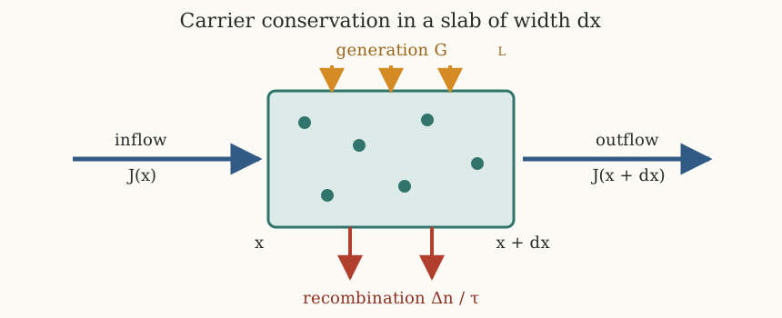
Carrier accumulation equals inflow minus outflow, plus optical generation, minus recombination.

The symbols used below are:

Symbol	Meaning	Units
\(\Delta n_p(x,t)\)	Excess minority-electron concentration in p-type material	\(\mathrm{cm^{-3}}\)
\(J(x)\)	Diffusion current density, using the book’s sign convention	\(\mathrm{A\,cm^{-2}}\)
\(D_e\)	Electron diffusion coefficient	\(\mathrm{cm^2\,s^{-1}}\)
\(\tau_e\)	Minority-electron recombination lifetime	\(\mathrm s\)
\(G_L\)	Optical generation rate per unit volume	\(\mathrm{cm^{-3}\,s^{-1}}\)

Step 1: A concentration gradient produces diffusion

Carriers diffuse from high concentration toward low concentration. The book writes the resulting current density as

\[J(x)=-qD_e\frac{\partial\Delta n_p}{\partial x}.\]

The chapter initially writes \(n(x)\) instead of \(\Delta n_p(x)\). In the neutral p-region,

\[n_p(x)=n_{p0}+\Delta n_p(x).\]

The equilibrium concentration \(n_{p0}\) is spatially constant, so

\[\frac{\partial n_p}{\partial x} =\frac{\partial\Delta n_p}{\partial x}.\]

The two notations therefore give the same diffusion term.

Step 2: Apply carrier conservation to a thin slab

Consider a slab extending from \(x\) to \(x+dx\).

• Current density entering the slab is \(J(x)\).

• Current density leaving it is \(J(x+dx)\).

Expand the outgoing current to first order:

\[J(x+dx) \approx J(x)+\frac{\partial J}{\partial x}dx.\]

The net carrier inflow per unit volume and time is consequently

\[\begin{split}\begin{aligned} \text{net inflow} &=\frac{J(x)-J(x+dx)}{q\,dx}\\ &=-\frac{1}{q}\frac{\partial J}{\partial x}. \end{aligned}\end{split}\]

This is the crucial extra derivative.

Step 3: Add generation and recombination

Three processes change the excess-carrier concentration:

\[\text{rate of change} = \text{net inflow} -\text{recombination} +\text{optical generation}.\]

In symbols,

\[\frac{\partial\Delta n_p}{\partial t} = -\frac{1}{q}\frac{\partial J}{\partial x} -\frac{\Delta n_p}{\tau_e} +G_L.\]

Step 4: Substitute the diffusion current

Insert \(J=-qD_e\,\partial\Delta n_p/\partial x\):

\[\begin{split}\begin{aligned} -\frac{1}{q}\frac{\partial J}{\partial x} &=-\frac{1}{q}\frac{\partial}{\partial x} \left( -qD_e\frac{\partial\Delta n_p}{\partial x} \right)\\ &=D_e\frac{\partial^2\Delta n_p}{\partial x^2}, \end{aligned}\end{split}\]

where \(D_e\) is assumed constant. The complete result is

\[\frac{\partial\Delta n_p}{\partial t} = D_e\frac{\partial^2\Delta n_p}{\partial x^2} -\frac{\Delta n_p}{\tau_e} +G_L. \tag{3.5}\]

Why it is second order

The derivative chain is

\[\boxed{ \Delta n_p \xrightarrow{\ \partial/\partial x\ } J \xrightarrow{\ -\partial/\partial x\ } \text{carrier accumulation} }.\]

Therefore:

• Equation 3.5 is second order in position \(x\).

• It is only first order in time \(t\).

• The second spatial derivative measures the curvature of the concentration profile, not simply its slope.

A useful physical reading is:

• constant concentration gives no diffusion current;

• a straight concentration profile gives constant current but no local accumulation;

• a curved concentration profile makes current vary with position, so some regions gain or lose carriers.

Unit check

Every term in Equation 3.5 must have units of concentration change per time:

\[\left[ D_e\frac{\partial^2\Delta n_p}{\partial x^2} \right] = \frac{\mathrm{cm^2}}{\mathrm s} \frac{\mathrm{cm^{-3}}}{\mathrm{cm^2}} = \mathrm{cm^{-3}\,s^{-1}}.\]

The recombination and generation terms have the same units:

\[\left[\frac{\Delta n_p}{\tau_e}\right] = [G_L] = \mathrm{cm^{-3}\,s^{-1}}.\]

Steady-state Equation 3.6

At steady state the concentration profile no longer changes with time:

\[\frac{\partial\Delta n_p}{\partial t}=0.\]

Equation 3.5 then becomes

\[\frac{d^2\Delta n_p}{dx^2} = \frac{\Delta n_p}{D_e\tau_e} -\frac{G_L}{D_e}. \tag{3.6}\]

In the dark, \(G_L=0\). Define the electron diffusion length

\[L_e=\sqrt{D_e\tau_e}.\]

The equation reduces to

\[\frac{d^2\Delta n_p}{dx^2} -\frac{\Delta n_p}{L_e^2}=0,\]

whose decaying solution in a long neutral region is

\[\Delta n_p(x)=\Delta n_p(0)e^{-x/L_e}.\]

Because the spatial equation is second order, two boundary conditions are needed. Typically the junction supplies \(\Delta n_p(0)\) and the excess concentration approaches zero far from the junction.

Source correction

Warning

The paragraph below Equation 3.5 says that Equation 3.4 is a second-order differential equation. Equation 3.4 is algebraic. The sentence should refer to Equation 3.5.

Continue interactively

Use the Photonics Essentials: Chapter 3 Interactive Physics Lab to change the diffusion coefficient, carrier lifetime, generation rate, and the other Chapter 3 variables while the corresponding curves update.