Chapter 1: Ray Optics
Source: Saleh and Teich, Fundamentals of Photonics, second edition, Chapter 1. Prompts are paraphrased. Distances and radii use the book’s sign convention; \(P(d)\) and \(L(f)\) denote free-space and thin-lens ray matrices.
In-text exercises
Exercise 1.1-1 — Snell’s law from stationary optical path
Brief solution
1. Method. The calculation uses optical path and Fermat’s principle, the stationary-value condition, the chain rule and square-root derivative, and the right-triangle definitions of sine.
2. Key step.
Substituting Equation (8) into Equation (7) gives the required law:
3. Answer.
Show detailed steps
Problem in our own words. A ray travels from a fixed point \(A\) in medium 1 to a fixed point \(B\) in medium 2, crossing their planar interface at a movable point \(P\). Show that making the optical path stationary with respect to \(P\) gives Snell’s law.
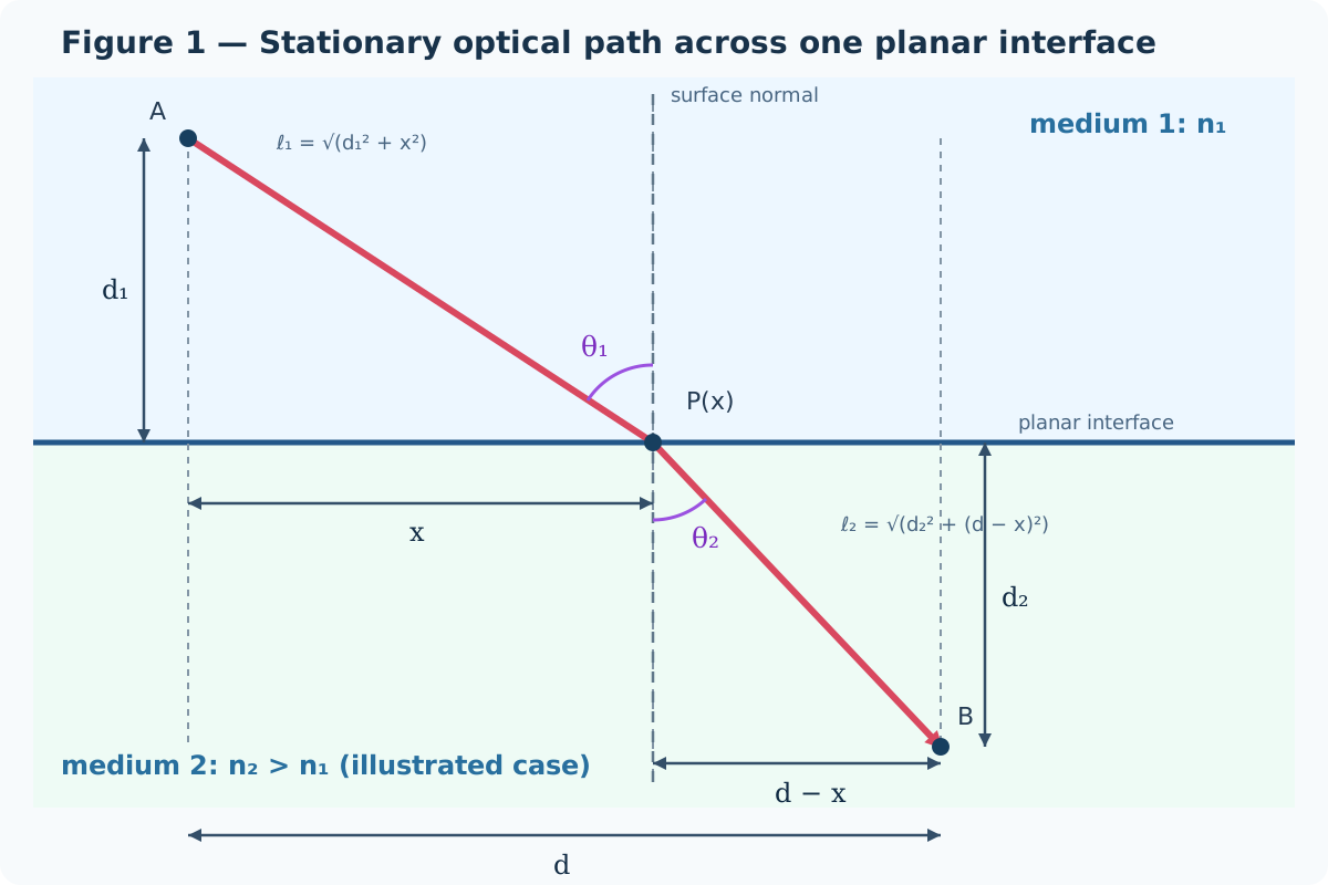
Figure 1 — Exercise 1.1-1: Snell’s law from stationary optical path. The crossing point has horizontal coordinate \(x\). Every geometrical variable used in the derivation is defined in the drawing.
Definitions and assumptions.
\(n_1,n_2\) are the constant refractive indices above and below the interface.
\(d_1,d_2>0\) are the perpendicular distances from \(A\) and \(B\) to the interface; \(d>0\) is their total horizontal separation.
\(x\) is the horizontal distance from the projection of \(A\) to \(P\), so the second horizontal leg is \(d-x\) and \(0<x<d\).
\(\ell_1,\ell_2\) are the two geometrical path lengths.
\(\theta_1,\theta_2\) are measured from the interface normal, not from the interface itself.
The media are homogeneous and isotropic, the interface is planar, and the endpoints are fixed. Reflections and any phase shift at the boundary do not affect the ray path being varied.
By the Pythagorean theorem, the segment lengths in the figure are
Mathematical formulas used. The calculation uses optical path and Fermat’s principle, the stationary-value condition, the chain rule and square-root derivative, and the right-triangle definitions of sine.
Step 1 — Write the quantity that must be stationary. In a homogeneous piece of medium, OPL equals refractive index times geometrical length. Therefore the total OPL through \(P(x)\) is
The transit time is \(T(x)=\mathcal L(x)/c\); since \(c\) is constant, \(dT/dx=0\) and \(d\mathcal L/dx=0\) are equivalent.
Step 2 — Differentiate every term explicitly. For the first square root, take \(u_1=d_1^2+x^2\). Then \(u_1'=2x\), so Equation (3) gives
For the second square root, let \(u_2=d_2^2+(d-x)^2\). The nested derivative is
The minus sign appears because moving \(P\) to the right lengthens the first horizontal leg but shortens the second. Applying the square-root rule again,
Combining Equations (3) and (5) yields
Step 3 — Impose stationarity. Fermat’s principle and Equation (4) require
where \(x_*\) is the physical crossing point.
Step 4 — Translate the geometrical ratios into angles. From the two right triangles in the SVG,
Substituting Equation (8) into Equation (7) gives the required law:
Checks. Both sides of Equation (9) are dimensionless. If \(n_1=n_2\), then \(\sin\theta_1=\sin\theta_2\); for angles between \(0\) and \(\pi/2\), this gives \(\theta_1=\theta_2\), so the two segments form one straight line. At normal incidence, \(x_*=0\) and \(d-x_*=0\) in the corresponding aligned geometry (\(d=0\)), and both sides vanish. These limits agree with physical expectation.
Exercise 1.2-1 — Spherical-mirror imaging
Brief solution
1. Method. The working uses trigonometric and small-angle identities and algebraic rearrangement and dimensional checks.
2. Reasoning and answer.
Show detailed steps
Step 1 — Definitions and setup. Symbols are local to this item and follow the chapter convention. Each physical quantity and supplied numerical value is introduced at its first use below; angles are in radians unless a degree symbol is shown, and units are retained through numerical substitution.
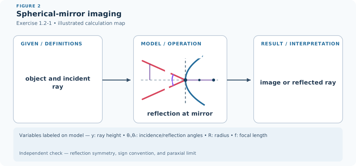
Figure 2 — Exercise 1.2-1: Spherical-mirror imaging. The diagram identifies the input quantities, physical operation, requested result, variable meanings, and an independent verification route. Every symbol in the variable strip is labeled on the model itself.
Step 2 — Mathematical formulas used. The working uses trigonometric and small-angle identities and algebraic rearrangement and dimensional checks.
Step 3 — Worked derivation. The calculation is kept in symbolic form until the governing relation has been rearranged for the requested quantity.
Detailed step 1. At height \(y\),
Detailed step 2. the paraxial surface normal has angle \(y/R\).
Detailed step 3. Reflection gives \((y-y_1)/z_1+(y-y_2)/z_2=2y/R\).
Detailed step 4. For the coefficient of the arbitrary intercept \(y\) to vanish, \(1/z_1+1/z_2=2/R=1/f\).
Detailed step 5. The remaining term gives \(y_2=-y_1z_2/z_1\); hence every ray from one object point reaches the same,
Detailed step 6. inverted image point.
Step 4 — State the numbered result. The principal result obtained in the working is
Step 5 — Check. Equation (10) can be checked by substituting it back into the preceding governing relation and reversing the algebraic steps. The zero-angle or paraxial limit supplies an independent sign and magnitude check whenever that limit is part of the model.
Exercise 1.2-2 — One spherical refracting boundary
Brief solution
1. Method. The working uses trigonometric and small-angle identities and algebraic rearrangement and dimensional checks.
2. Key step.
Paraxial Snell refraction at height \(y\) gives \(n_1(y-y_1)/z_1+n_2(y_2-y)/z_2=(n_2-n_1)y/R\). Equating the coefficient and constant terms yields
3. Answer.
Show detailed steps
Step 1 — Definitions and setup. Symbols are local to this item and follow the chapter convention. Each physical quantity and supplied numerical value is introduced at its first use below; angles are in radians unless a degree symbol is shown, and units are retained through numerical substitution.
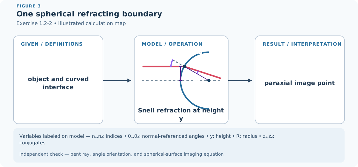
Figure 3 — Exercise 1.2-2: One spherical refracting boundary. The diagram identifies the input quantities, physical operation, requested result, variable meanings, and an independent verification route. Every symbol in the variable strip is labeled on the model itself.
Step 2 — Mathematical formulas used. The working uses trigonometric and small-angle identities and algebraic rearrangement and dimensional checks.
Step 3 — Worked derivation. The calculation is kept in symbolic form until the governing relation has been rearranged for the requested quantity.
Paraxial Snell refraction at height \(y\) gives \(n_1(y-y_1)/z_1+n_2(y_2-y)/z_2=(n_2-n_1)y/R\). Equating the coefficient and constant terms yields
Step 4 — Interpret the result. The final relation or conclusion in Step 3 is the requested result. Read its sign, scale, or physical classification using the conventions fixed in Step 1.
Step 5 — Check. Equation (11) can be checked by substituting it back into the preceding governing relation and reversing the algebraic steps. The zero-angle or paraxial limit supplies an independent sign and magnitude check whenever that limit is part of the model.
Exercise 1.2-3 — Aberration-free refracting surface
Brief solution
1. Method. The working uses optical path and Fermat’s principle and algebraic rearrangement and dimensional checks.
2. Key step.
Let a surface point be \((y,z)\), with the two axial conjugates at \((0,-z_1)\) and \((0,z_2)\). Fermat’s principle requires
3. Answer.
This Cartesian oval, not a sphere in general, makes the optical path identical for every ray and therefore images without spherical aberration.
Show detailed steps
Step 1 — Definitions and setup. Symbols are local to this item and follow the chapter convention. Each physical quantity and supplied numerical value is introduced at its first use below; angles are in radians unless a degree symbol is shown, and units are retained through numerical substitution.
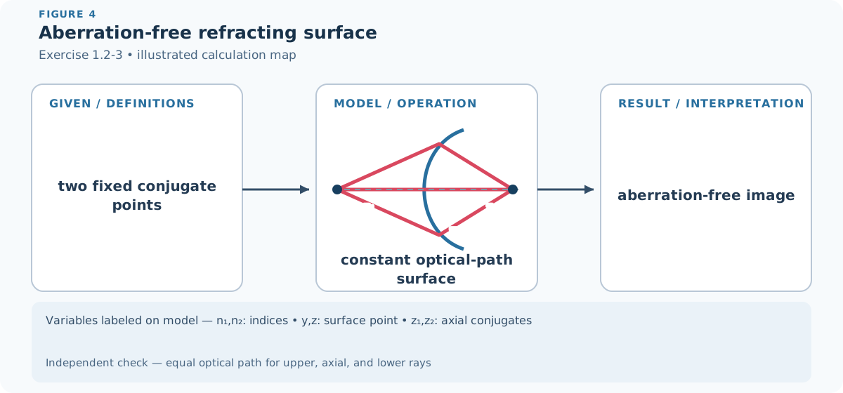
Figure 4 — Exercise 1.2-3: Aberration-free refracting surface. The diagram identifies the input quantities, physical operation, requested result, variable meanings, and an independent verification route. Every symbol in the variable strip is labeled on the model itself.
Step 2 — Mathematical formulas used. The working uses optical path and Fermat’s principle and algebraic rearrangement and dimensional checks.
Step 3 — Worked derivation. The calculation is kept in symbolic form until the governing relation has been rearranged for the requested quantity.
Let a surface point be \((y,z)\), with the two axial conjugates at \((0,-z_1)\) and \((0,z_2)\). Fermat’s principle requires
This Cartesian oval, not a sphere in general, makes the optical path identical for every ray and therefore images without spherical aberration.
Step 4 — Interpret the result. The final relation or conclusion in Step 3 is the requested result. Read its sign, scale, or physical classification using the conventions fixed in Step 1.
Step 5 — Check. Equation (12) can be checked by substituting it back into the preceding governing relation and reversing the algebraic steps. Check that dimensions agree term by term, then test the simplest symmetry or limiting case for the expected sign and scale.
Exercise 1.2-4 — Thin-lens formulas
Brief solution
1. Method. The working uses algebraic rearrangement and dimensional checks.
2. Key step.
Apply the preceding boundary equation first at \(R_1\), then at \(R_2\), and let the center thickness tend to zero. The intermediate image distance cancels, leaving
3. Answer.
Show detailed steps
Step 1 — Definitions and setup. Symbols are local to this item and follow the chapter convention. Each physical quantity and supplied numerical value is introduced at its first use below; angles are in radians unless a degree symbol is shown, and units are retained through numerical substitution.
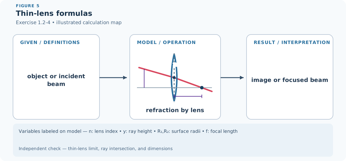
Figure 5 — Exercise 1.2-4: Thin-lens formulas. The diagram identifies the input quantities, physical operation, requested result, variable meanings, and an independent verification route. Every symbol in the variable strip is labeled on the model itself.
Step 2 — Mathematical formulas used. The working uses algebraic rearrangement and dimensional checks.
Step 3 — Worked derivation. The calculation is kept in symbolic form until the governing relation has been rearranged for the requested quantity.
Apply the preceding boundary equation first at \(R_1\), then at \(R_2\), and let the center thickness tend to zero. The intermediate image distance cancels, leaving
Step 4 — Interpret the result. The final relation or conclusion in Step 3 is the requested result. Read its sign, scale, or physical classification using the conventions fixed in Step 1.
Step 5 — Check. Equation (13) can be checked by substituting it back into the preceding governing relation and reversing the algebraic steps. Check that dimensions agree term by term, then test the simplest symmetry or limiting case for the expected sign and scale.
Exercise 1.2-5 — Step-index fibre acceptance
Brief solution
1. Method. The working uses trigonometric and small-angle identities and algebraic rearrangement and dimensional checks.
2. Key step.
At the core-cladding boundary, the limiting ray obeys \(\sin\theta_c=n_2/n_1\). Geometry gives \(\sin\theta_z=\cos\theta_c\); applying Snell’s law at the input face then gives
3. Answer.
Show detailed steps
Step 1 — Definitions and setup. Symbols are local to this item and follow the chapter convention. Each physical quantity and supplied numerical value is introduced at its first use below; angles are in radians unless a degree symbol is shown, and units are retained through numerical substitution.
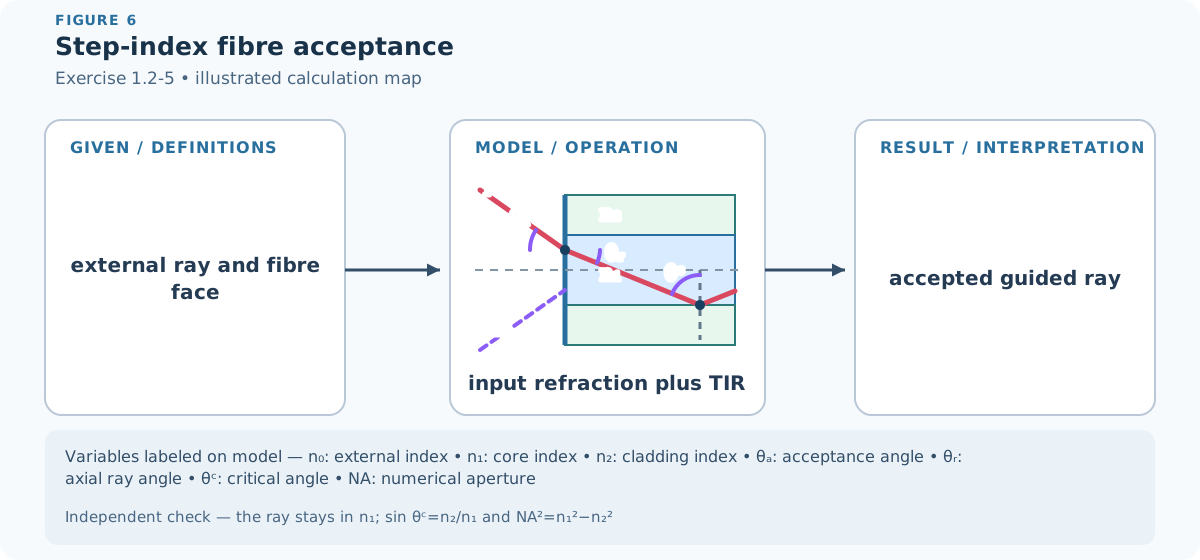
Figure 6 — Exercise 1.2-5: Step-index fibre acceptance. The diagram identifies the input quantities, physical operation, requested result, variable meanings, and an independent verification route. Every symbol in the variable strip is labeled on the model itself.
Step 2 — Mathematical formulas used. The working uses trigonometric and small-angle identities and algebraic rearrangement and dimensional checks.
Step 3 — Worked derivation. The calculation is kept in symbolic form until the governing relation has been rearranged for the requested quantity.
At the core-cladding boundary, the limiting ray obeys \(\sin\theta_c=n_2/n_1\). Geometry gives \(\sin\theta_z=\cos\theta_c\); applying Snell’s law at the input face then gives
Step 4 — Interpret the result. The final relation or conclusion in Step 3 is the requested result. Read its sign, scale, or physical classification using the conventions fixed in Step 1.
Step 5 — Check. Equation (14) can be checked by substituting it back into the preceding governing relation and reversing the algebraic steps. The zero-angle or paraxial limit supplies an independent sign and magnitude check whenever that limit is part of the model. Repeat the substitution with unrounded intermediate values and retain the displayed units; the final unit must have the requested dimension.
Exercise 1.2-6 — Light trapped in a high-index block
Brief solution
1. Method. The working uses Snell’s law and the trigonometric identities, the solid angle of a circular cone, and algebraic rearrangement and limiting checks.
2. Key step.
3. Answer.
Show detailed steps
Step 1 — Definitions and setup. A rectangular parallelepiped of refractive index \(n\) is surrounded by air (\(n_{\mathrm{out}}=1\)). Light is generated isotropically inside it. We shall answer the two requested parts separately.
\(\theta_i\) is a ray’s incidence angle, measured from the outward normal to the face that it reaches.
\(\theta_c\) is the critical angle and therefore the half-angle of one face’s internal escape cone. The cone’s full apex angle is \(2\theta_c\).
\(\Omega_c\) is the solid angle of one escape cone.
\(P_{\mathrm{ext}}/P_{\mathrm{tot}}\) is the fraction of the isotropically generated power lying in all escape cones.
The calculation uses ideal geometrical optics: the faces are perfectly parallel, and absorption, scattering, and Fresnel reflection below the critical angle are neglected. Thus part (b) gives the maximum geometrical extraction fraction under the exercise’s assumptions.
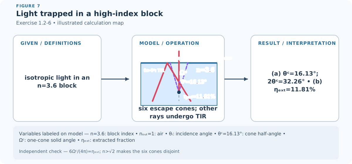
Figure 7 — Exercise 1.2-6: Light trapped in a high-index block. The diagram identifies the input quantities, physical operation, requested result, variable meanings, and an independent verification route. Every symbol in the variable strip is labeled on the model itself.
Step 2 — Mathematical formulas used. The working uses Snell’s law and the trigonometric identities, the solid angle of a circular cone, and algebraic rearrangement and limiting checks.
Step 3 — Worked derivation.
(a) Escape cone and trapped rays. At the limiting ray, the transmitted angle is \(\theta_t=90^\circ\). Snell’s law at an interior-to-air face therefore becomes
Rays with \(0\leq\theta_i<\theta_c\) lie inside that face’s escape cone and refract into air. Rays with \(\theta_i>\theta_c\) undergo total internal reflection. In the ideal parallel-sided block, directions outside all six escape cones continue to reflect and remain trapped. The equality \(\theta_i=\theta_c\) is the limiting ray traveling along the surface.
For GaAs, \(n=3.6\), so the cone half-angle and full apex angle are
(b) Extracted-power fraction. For an isotropic source, power per unit solid angle is constant. Integrating over the circular cone about one face normal gives
The six face normals occur in three opposite pairs and adjacent normals are separated by \(90^\circ\). The condition \(n>\sqrt2\) gives \(\theta_c<45^\circ\), so adjacent escape cones do not overlap. Their solid angles can therefore be added without double counting:
Here we used the positive root because \(0<\theta_c<90^\circ\). Substitution for GaAs gives
Step 4 — State the numbered results. Both requested answers are
Step 5 — Checks.
Substitution gives \(3.6\sin(16.1276^\circ)=1.00000\), as required for a critical ray at a GaAs-air boundary.
One cone occupies \(\Omega_c=0.24727\ \mathrm{sr}\); six cones occupy \(1.48364\ \mathrm{sr}\). Dividing by \(4\pi=12.56637\ \mathrm{sr}\) again gives \(0.118064\).
Since \(3.6>\sqrt2\), the GaAs half-angle is less than \(45^\circ\); hence the six-cone, no-overlap assumption is valid.
For large \(n\), the square-root expansion gives \(P_{\mathrm{ext}}/P_{\mathrm{tot}}\simeq3/(2n^2)\). At \(n=3.6\) this is \(0.1157\), close to the exact \(0.1181\) and of the expected small magnitude.
Exercise 1.3-1 — A SELFOC slab as a lens
Brief solution
1. Method. The working uses common differential-equation solutions, trigonometric and small-angle identities, and algebraic rearrangement and dimensional checks.
2. Key step.
For \(n(y)\simeq n_0(1-a^2y^2/2)\), the paraxial ray equation is \(y''+a^2y=0\). Propagating its sine-cosine solution through length \(d\) and extending the exit tangent to the axis gives
3. Answer.
At \(d=\pi/(2a)\) all rays cross the axis at the exit quarter-pitch; at \(d=\pi/a\) they form an inverted unit-magnification half-pitch image.
Show detailed steps
Step 1 — Definitions and setup. Symbols are local to this item and follow the chapter convention. Each physical quantity and supplied numerical value is introduced at its first use below; angles are in radians unless a degree symbol is shown, and units are retained through numerical substitution.
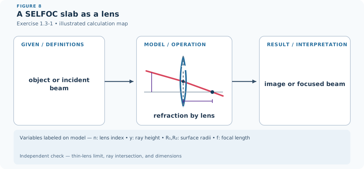
Figure 8 — Exercise 1.3-1: A SELFOC slab as a lens. The diagram identifies the input quantities, physical operation, requested result, variable meanings, and an independent verification route. Every symbol in the variable strip is labeled on the model itself.
Step 2 — Mathematical formulas used. The working uses common differential-equation solutions, trigonometric and small-angle identities, and algebraic rearrangement and dimensional checks.
Step 3 — Worked derivation. The calculation is kept in symbolic form until the governing relation has been rearranged for the requested quantity.
For \(n(y)\simeq n_0(1-a^2y^2/2)\), the paraxial ray equation is \(y''+a^2y=0\). Propagating its sine-cosine solution through length \(d\) and extending the exit tangent to the axis gives
At \(d=\pi/(2a)\) all rays cross the axis at the exit quarter-pitch; at \(d=\pi/a\) they form an inverted unit-magnification half-pitch image.
Step 4 — Interpret the result. The final relation or conclusion in Step 3 is the requested result. Read its sign, scale, or physical classification using the conventions fixed in Step 1.
Step 5 — Check. Equation (21) can be checked by substituting it back into the preceding governing relation and reversing the algebraic steps. The zero-angle or paraxial limit supplies an independent sign and magnitude check whenever that limit is part of the model.
Exercise 1.3-2 — Graded-index fibre acceptance
Brief solution
1. Method. The working uses trigonometric and small-angle identities and algebraic rearrangement and dimensional checks.
2. Reasoning and answer.
Show detailed steps
Step 1 — Definitions and setup. Symbols are local to this item and follow the chapter convention. Each physical quantity and supplied numerical value is introduced at its first use below; angles are in radians unless a degree symbol is shown, and units are retained through numerical substitution.
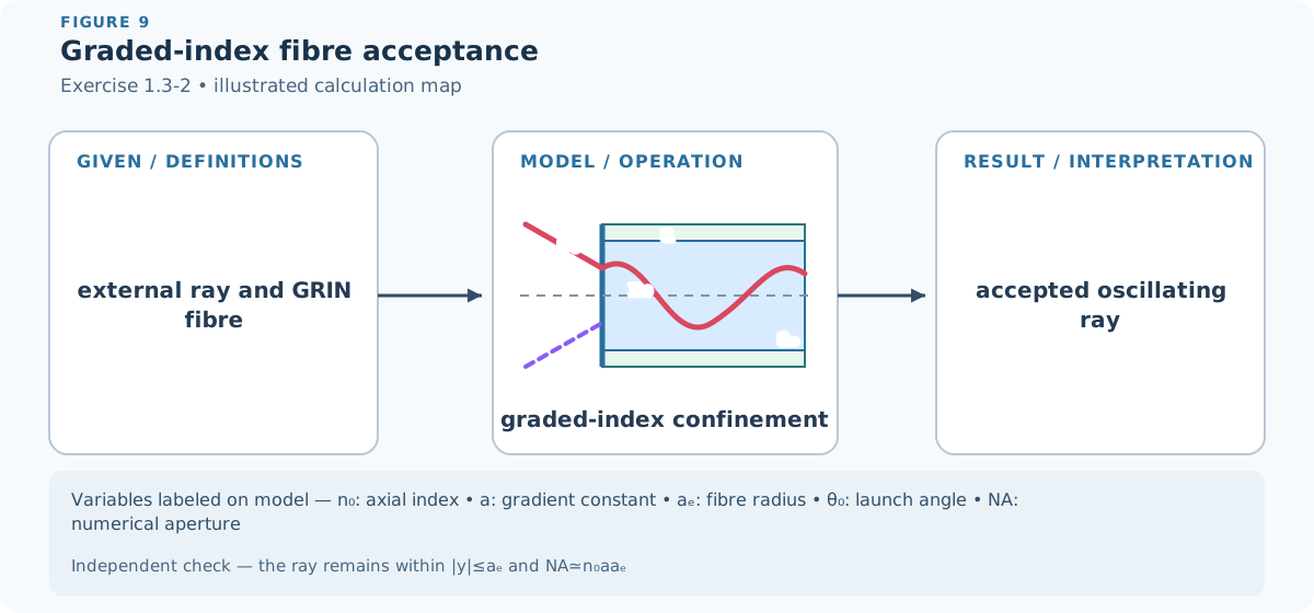
Figure 9 — Exercise 1.3-2: Graded-index fibre acceptance. The diagram identifies the input quantities, physical operation, requested result, variable meanings, and an independent verification route. Every symbol in the variable strip is labeled on the model itself.
Step 2 — Mathematical formulas used. The working uses trigonometric and small-angle identities and algebraic rearrangement and dimensional checks.
Step 3 — Worked derivation. The calculation is kept in symbolic form until the governing relation has been rearranged for the requested quantity.
Detailed step 1. The conserved paraxial ray energy is \((y')^2+a^2y^2=\theta_0^2\).
Detailed step 2. Confinement to \(|y|\leq a_f\) requires \(\theta_0\leq aa_f\); input-face Snell refraction therefore gives \(\boxed{\mathrm{NA}\simeq n_0aa_f}\).
Detailed step 3. Since \(n(a_f)\simeq n_0(1-a^2a_f^2/2)\),
Detailed step 4. the matched step-index result \(\sqrt{n_0^2-n(a_f)^2}\) has the same first-order value.
Step 4 — State the numbered result. The principal result obtained in the working is
Step 5 — Check. Equation (22) can be checked by substituting it back into the preceding governing relation and reversing the algebraic steps. The zero-angle or paraxial limit supplies an independent sign and magnitude check whenever that limit is part of the model. Repeat the substitution with unrounded intermediate values and retain the displayed units; the final unit must have the requested dimension.
Exercise 1.4-1 — Zero elements of an ABCD matrix
Brief solution
1. Method. The working uses matrix multiplication and eigenvalue rules, trigonometric and small-angle identities, and algebraic rearrangement and dimensional checks.
2. Key step.
From \(y_2=Ay_1+B\theta_1\) and \(\theta_2=Cy_1+D\theta_1\): \(A=0\) maps equal input angles to one output height; \(B=0\) images an input plane; \(C=0\) is afocal; and \(D=0\) maps equal input heights to one output angle.
3. Answer.
Show detailed steps
Step 1 — Definitions and setup. Symbols are local to this item and follow the chapter convention. Each physical quantity and supplied numerical value is introduced at its first use below; angles are in radians unless a degree symbol is shown, and units are retained through numerical substitution.
Figure 10 — Exercise 1.4-1: Zero elements of an ABCD matrix. The diagram identifies the input quantities, physical operation, requested result, variable meanings, and an independent verification route. Every symbol in the variable strip is labeled on the model itself.
Step 2 — Mathematical formulas used. The working uses matrix multiplication and eigenvalue rules, trigonometric and small-angle identities, and algebraic rearrangement and dimensional checks.
Step 3 — Worked derivation. The calculation is kept in symbolic form until the governing relation has been rearranged for the requested quantity.
From \(y_2=Ay_1+B\theta_1\) and \(\theta_2=Cy_1+D\theta_1\): \(A=0\) maps equal input angles to one output height; \(B=0\) images an input plane; \(C=0\) is afocal; and \(D=0\) maps equal input heights to one output angle.
Step 4 — State the numbered result. The principal result obtained in the working is
Step 5 — Check. Equation (23) can be checked by substituting it back into the preceding governing relation and reversing the algebraic steps. Multiply the matrices independently in the stated input-to-output order and verify that every product has compatible dimensions.
Exercise 1.4-2 — Parallel plates
Brief solution
1. Method. The working uses matrix multiplication and eigenvalue rules, trigonometric and small-angle identities, and algebraic rearrangement and dimensional checks.
2. Key step.
Using reduced angle \(n\theta\), each plate is \(\begin{bmatrix}1&d_i/n_i\\0&1\end{bmatrix}\). Such shear matrices add, so
3. Answer.
Show detailed steps
Step 1 — Definitions and setup. Symbols are local to this item and follow the chapter convention. Each physical quantity and supplied numerical value is introduced at its first use below; angles are in radians unless a degree symbol is shown, and units are retained through numerical substitution.
Figure 11 — Exercise 1.4-2: Parallel plates. The diagram identifies the input quantities, physical operation, requested result, variable meanings, and an independent verification route. Every symbol in the variable strip is labeled on the model itself.
Step 2 — Mathematical formulas used. The working uses matrix multiplication and eigenvalue rules, trigonometric and small-angle identities, and algebraic rearrangement and dimensional checks.
Step 3 — Worked derivation. The calculation is kept in symbolic form until the governing relation has been rearranged for the requested quantity.
Using reduced angle \(n\theta\), each plate is \(\begin{bmatrix}1&d_i/n_i\\0&1\end{bmatrix}\). Such shear matrices add, so
Step 4 — Interpret the result. The final relation or conclusion in Step 3 is the requested result. Read its sign, scale, or physical classification using the conventions fixed in Step 1.
Step 5 — Check. Equation (24) can be checked by substituting it back into the preceding governing relation and reversing the algebraic steps. Multiply the matrices independently in the stated input-to-output order and verify that every product has compatible dimensions.
Exercise 1.4-3 — Gap followed by a lens
Brief solution
1. Method. The working uses matrix multiplication and eigenvalue rules and algebraic rearrangement and dimensional checks.
2. Key step.
Direct multiplication gives
3. Answer.
Show detailed steps
Step 1 — Definitions and setup. Symbols are local to this item and follow the chapter convention. Each physical quantity and supplied numerical value is introduced at its first use below; angles are in radians unless a degree symbol is shown, and units are retained through numerical substitution.
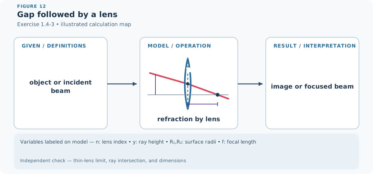
Figure 12 — Exercise 1.4-3: Gap followed by a lens. The diagram identifies the input quantities, physical operation, requested result, variable meanings, and an independent verification route. Every symbol in the variable strip is labeled on the model itself.
Step 2 — Mathematical formulas used. The working uses matrix multiplication and eigenvalue rules and algebraic rearrangement and dimensional checks.
Step 3 — Worked derivation. The calculation is kept in symbolic form until the governing relation has been rearranged for the requested quantity.
Direct multiplication gives
Step 4 — Interpret the result. The final relation or conclusion in Step 3 is the requested result. Read its sign, scale, or physical classification using the conventions fixed in Step 1.
Step 5 — Check. Equation (25) can be checked by substituting it back into the preceding governing relation and reversing the algebraic steps. Multiply the matrices independently in the stated input-to-output order and verify that every product has compatible dimensions.
Exercise 1.4-4 — Single-lens imaging
Brief solution
1. Method. The working uses trigonometric and small-angle identities and algebraic rearrangement and dimensional checks.
2. Reasoning and answer.
Show detailed steps
Step 1 — Definitions and setup. Symbols are local to this item and follow the chapter convention. Each physical quantity and supplied numerical value is introduced at its first use below; angles are in radians unless a degree symbol is shown, and units are retained through numerical substitution.
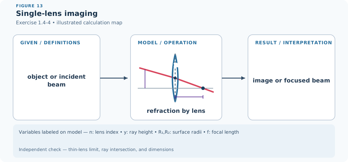
Figure 13 — Exercise 1.4-4: Single-lens imaging. The diagram identifies the input quantities, physical operation, requested result, variable meanings, and an independent verification route. Every symbol in the variable strip is labeled on the model itself.
Step 2 — Mathematical formulas used. The working uses trigonometric and small-angle identities and algebraic rearrangement and dimensional checks.
Step 3 — Worked derivation. The calculation is kept in symbolic form until the governing relation has been rearranged for the requested quantity.
Detailed step 1. For \(M=P(d_2)L(f)P(d_1)\),
Detailed step 2. the element \(B=d_1+d_2-d_1d_2/f\).
Detailed step 3. The imaging law makes \(B=0\),
Detailed step 4. so \(y_2=Ay_1=-(d_2/d_1)y_1\),
Detailed step 5. independently of input angle.
Detailed step 6. Setting \(d_2=f\) instead makes \(A=0\),
Detailed step 7. so all rays of one input angle meet at \(y_2=f\theta_1\).
Step 4 — State the numbered result. The principal result obtained in the working is
Step 5 — Check. Equation (26) can be checked by substituting it back into the preceding governing relation and reversing the algebraic steps. The zero-angle or paraxial limit supplies an independent sign and magnitude check whenever that limit is part of the model.
Exercise 1.4-5 — Thick symmetric lens
Brief solution
1. Method. The working uses algebraic rearrangement and dimensional checks.
2. Key step.
Multiplying the two spherical refractions and the internal translation gives the equivalent power
3. Answer.
Locating the principal planes from the resulting \(A,D\) elements changes the vertex distances to \(z_1=d_1+h_1\) and \(z_2=d_2+h_2\). The condition \(B=0\) then reduces to \(1/z_1+1/z_2=1/f\), which proves the stated thick-lens form.
Show detailed steps
Step 1 — Definitions and setup. Symbols are local to this item and follow the chapter convention. Each physical quantity and supplied numerical value is introduced at its first use below; angles are in radians unless a degree symbol is shown, and units are retained through numerical substitution.
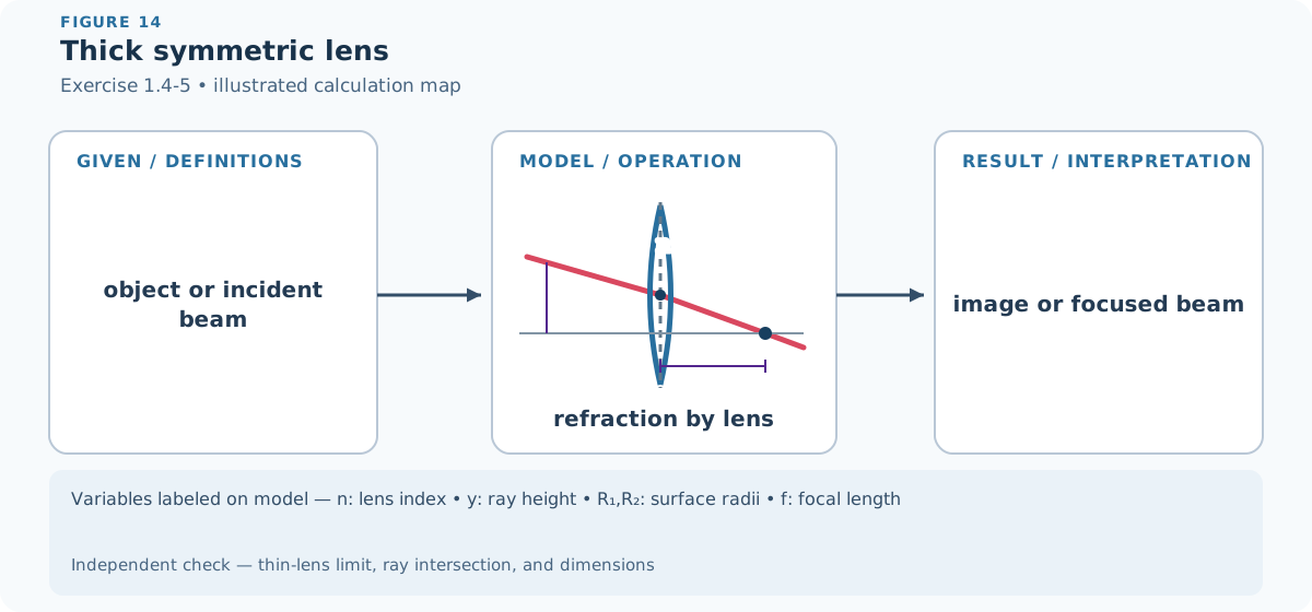
Figure 14 — Exercise 1.4-5: Thick symmetric lens. The diagram identifies the input quantities, physical operation, requested result, variable meanings, and an independent verification route. Every symbol in the variable strip is labeled on the model itself.
Step 2 — Mathematical formulas used. The working uses algebraic rearrangement and dimensional checks.
Step 3 — Worked derivation. The calculation is kept in symbolic form until the governing relation has been rearranged for the requested quantity.
Multiplying the two spherical refractions and the internal translation gives the equivalent power
Locating the principal planes from the resulting \(A,D\) elements changes the vertex distances to \(z_1=d_1+h_1\) and \(z_2=d_2+h_2\). The condition \(B=0\) then reduces to \(1/z_1+1/z_2=1/f\), which proves the stated thick-lens form.
Step 4 — Interpret the result. The final relation or conclusion in Step 3 is the requested result. Read its sign, scale, or physical classification using the conventions fixed in Step 1.
Step 5 — Check. Equation (27) can be checked by substituting it back into the preceding governing relation and reversing the algebraic steps. Check that dimensions agree term by term, then test the simplest symmetry or limiting case for the expected sign and scale.
Exercise 1.4-6 — Alternating periodic lenses
Brief solution
1. Method. The working uses algebraic rearrangement and dimensional checks.
2. Key step.
Multiply one complete cell and apply the unimodular stability test \(|\operatorname{tr}M/2|<1\). The trace simplifies to
3. Answer.
Show detailed steps
Step 1 — Definitions and setup. Symbols are local to this item and follow the chapter convention. Each physical quantity and supplied numerical value is introduced at its first use below; angles are in radians unless a degree symbol is shown, and units are retained through numerical substitution.
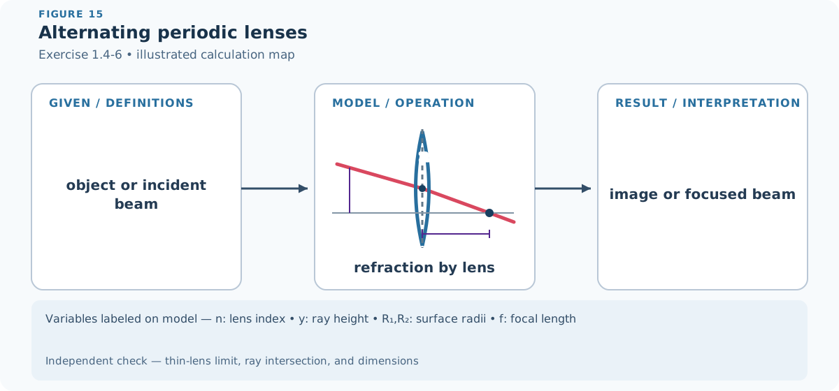
Figure 15 — Exercise 1.4-6: Alternating periodic lenses. The diagram identifies the input quantities, physical operation, requested result, variable meanings, and an independent verification route. Every symbol in the variable strip is labeled on the model itself.
Step 2 — Mathematical formulas used. The working uses algebraic rearrangement and dimensional checks.
Step 3 — Worked derivation. The calculation is kept in symbolic form until the governing relation has been rearranged for the requested quantity.
Multiply one complete cell and apply the unimodular stability test \(|\operatorname{tr}M/2|<1\). The trace simplifies to
Step 4 — Interpret the result. The final relation or conclusion in Step 3 is the requested result. Read its sign, scale, or physical classification using the conventions fixed in Step 1.
Step 5 — Check. Equation (28) can be checked by substituting it back into the preceding governing relation and reversing the algebraic steps. Check that dimensions agree term by term, then test the simplest symmetry or limiting case for the expected sign and scale.
Exercise 1.4-7 — Two-mirror resonator
Brief solution
1. Method. The working uses matrix multiplication and eigenvalue rules and algebraic rearrangement and dimensional checks.
Show detailed steps
Step 1 — Definitions and setup. Symbols are local to this item and follow the chapter convention. Each physical quantity and supplied numerical value is introduced at its first use below; angles are in radians unless a degree symbol is shown, and units are retained through numerical substitution.
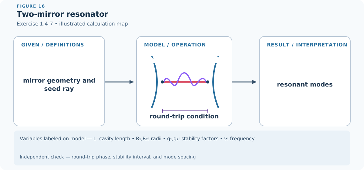
Figure 16 — Exercise 1.4-7: Two-mirror resonator. The diagram identifies the input quantities, physical operation, requested result, variable meanings, and an independent verification route. Every symbol in the variable strip is labeled on the model itself.
Step 2 — Mathematical formulas used. The working uses matrix multiplication and eigenvalue rules and algebraic rearrangement and dimensional checks.
Step 3 — Worked derivation. The calculation is kept in symbolic form until the governing relation has been rearranged for the requested quantity.
Detailed step 1. The round-trip matrix is the product of two translations and two mirror powers.
Detailed step 2. With \(g_i=1+d/R_i\) in the book’s radius convention, \((\operatorname{tr}M+2)/4=g_1g_2\).
Detailed step 3. Hence bounded rays require \(\boxed{0<g_1g_2<1}\) (equality is marginal).
End-of-chapter problems
Step 4 — State the numbered result. The principal result obtained in the working is
Step 5 — Check. Equation (29) can be checked by substituting it back into the preceding governing relation and reversing the algebraic steps. Multiply the matrices independently in the stated input-to-output order and verify that every product has compatible dimensions.
Problem 1.1-2 — Stationary time need not be a minimum
Brief solution
1. Method. The working uses stationary-value condition and optical path and Fermat’s principle.
Show detailed steps
Definitions and setup. Symbols are local to this item and follow the chapter convention. Each physical quantity and supplied numerical value is introduced at its first use below; angles are in radians unless a degree symbol is shown, and units are retained through numerical substitution.
Mathematical formulas used. The working uses stationary-value condition and optical path and Fermat’s principle.
Worked derivation. The calculation is kept in symbolic form until the governing relation has been rearranged for the requested quantity.
Detailed step 1. The ellipse has constant \(AP+PB\); its first variation at the tangent point is zero.
Detailed step 2. An internally tangent surface lies inside the ellipse nearby,
Detailed step 3. so its adjacent broken paths are shorter and \(P\) is a local maximum.
Detailed step 4. A surface crossing the ellipse lies on opposite sides on either side of \(P\); the path difference changes sign,
Detailed step 5. making the stationary path an inflection.
Detailed step 6. Fermat’s principle therefore means stationary,
Detailed step 7. not always minimum,
Detailed step 8. time.
Check. Check that dimensions agree term by term, then test the simplest symmetry or limiting case for the expected sign and scale.
Problem 1.2-7 — Plane-parallel plate or stack
Brief solution
1. Method. The working uses trigonometric and small-angle identities and algebraic rearrangement and dimensional checks.
2. Key step.
Snell gives \(\sin\theta=n_1\sin\theta_1\) at entry and the reverse at exit, so the emergent angle is \(\theta\). Geometry gives the lateral shift
3. Answer.
For a stack, tangential wavevector conservation gives \(n_m\sin\theta_m=\sin\theta\) in every layer and the last boundary again returns angle \(\theta\); the individual lateral shifts add.
Show detailed steps
Definitions and setup. Symbols are local to this item and follow the chapter convention. Each physical quantity and supplied numerical value is introduced at its first use below; angles are in radians unless a degree symbol is shown, and units are retained through numerical substitution.
Mathematical formulas used. The working uses trigonometric and small-angle identities and algebraic rearrangement and dimensional checks.
Worked derivation. The calculation is kept in symbolic form until the governing relation has been rearranged for the requested quantity.
Snell gives \(\sin\theta=n_1\sin\theta_1\) at entry and the reverse at exit, so the emergent angle is \(\theta\). Geometry gives the lateral shift
For a stack, tangential wavevector conservation gives \(n_m\sin\theta_m=\sin\theta\) in every layer and the last boundary again returns angle \(\theta\); the individual lateral shifts add.
Check. Equation (30) can be checked by substituting it back into the preceding governing relation and reversing the algebraic steps. The zero-angle or paraxial limit supplies an independent sign and magnitude check whenever that limit is part of the model.
Problem 1.2-8 — Biconvex lens in air and water
Brief solution
1. Method. The working uses algebraic rearrangement and dimensional checks.
2. Key step.
For \(R_1=0.20\ \mathrm m\), \(R_2=-0.30\ \mathrm m\),
3. Answer.
Thus \(f_{air}=1/[0.5(5+3.333)]=\boxed{0.240\ \mathrm m}\). In water (\(n_m=4/3\)), \(n_l/n_m=1.125\), giving \(\boxed{f_{water}=0.960\ \mathrm m}\).
Show detailed steps
Definitions and setup. Symbols are local to this item and follow the chapter convention. Each physical quantity and supplied numerical value is introduced at its first use below; angles are in radians unless a degree symbol is shown, and units are retained through numerical substitution.
Mathematical formulas used. The working uses algebraic rearrangement and dimensional checks.
Worked derivation. The calculation is kept in symbolic form until the governing relation has been rearranged for the requested quantity.
For \(R_1=0.20\ \mathrm m\), \(R_2=-0.30\ \mathrm m\),
Thus \(f_{air}=1/[0.5(5+3.333)]=\boxed{0.240\ \mathrm m}\). In water (\(n_m=4/3\)), \(n_l/n_m=1.125\), giving \(\boxed{f_{water}=0.960\ \mathrm m}\).
Check. Equation (31) can be checked by substituting it back into the preceding governing relation and reversing the algebraic steps. Check that dimensions agree term by term, then test the simplest symmetry or limiting case for the expected sign and scale. Repeat the substitution with unrounded intermediate values and retain the displayed units; the final unit must have the requested dimension.
Problem 1.2-9 — Cladless fibre
Brief solution
1. Method. The working uses algebraic rearrangement and dimensional checks.
2. Reasoning and answer.
Show detailed steps
Definitions and setup. Symbols are local to this item and follow the chapter convention. Each physical quantity and supplied numerical value is introduced at its first use below; angles are in radians unless a degree symbol is shown, and units are retained through numerical substitution.
Mathematical formulas used. The working uses algebraic rearrangement and dimensional checks.
Worked derivation. The calculation is kept in symbolic form until the governing relation has been rearranged for the requested quantity.
Detailed step 1. \(\mathrm{NA}=\sqrt{1.46^2-1^2}=1.0647\).
Detailed step 2. Since an external numerical aperture cannot exceed one,
Detailed step 3. every ray in the incident air hemisphere can in principle be accepted: \(\boxed{\theta_a=90^\circ}\).
Detailed step 4. The value above one signals saturation,
Detailed step 5. not a sine larger than one.
Numbered result. The principal result obtained in the working is
Check. Equation (32) can be checked by substituting it back into the preceding governing relation and reversing the algebraic steps. Check that dimensions agree term by term, then test the simplest symmetry or limiting case for the expected sign and scale. Repeat the substitution with unrounded intermediate values and retain the displayed units; the final unit must have the requested dimension.
Problem 1.2-10 — Spherical coupling lens
Brief solution
1. Method. The working uses vector-calculus identities, trigonometric and small-angle identities, and algebraic rearrangement and dimensional checks.
2. Reasoning and answer.
Show detailed steps
Definitions and setup. Symbols are local to this item and follow the chapter convention. Each physical quantity and supplied numerical value is introduced at its first use below; angles are in radians unless a degree symbol is shown, and units are retained through numerical substitution.
Mathematical formulas used. The working uses vector-calculus identities, trigonometric and small-angle identities, and algebraic rearrangement and dimensional checks.
Worked derivation. The calculation is kept in symbolic form until the governing relation has been rearranged for the requested quantity.
Detailed step 1. Trace the ray through the two spherical interfaces with vector Snell refraction.
Detailed step 2. At the first hit \((z,y)=(-\sqrt{1-0.7^2},0.7)\) mm; applying \(n=1\rightarrow1.8\),
Detailed step 3. intersecting the far sphere,
Detailed step 4. and applying \(1.8\rightarrow1\) gives the second hit \((z,y)=(0.999725,0.023451)\) mm and emergent direction \((l,m)=(0.730362,-0.683060)\).
Detailed step 5. Its axial intercept is \(z=1.024800\) mm,
Detailed step 6. hence \(\boxed{f=0.02480\ \mathrm{mm}}\) beyond the rear vertex.
Detailed step 7. This exact meridional trace is preferable to the paraxial ball-lens BFL \(na/[2(n-1)]-a=0.125\ \mathrm{mm}\) because \(y/a=0.7\) is far outside the paraxial region.
Numbered result. The principal result obtained in the working is
Check. Equation (33) can be checked by substituting it back into the preceding governing relation and reversing the algebraic steps. The zero-angle or paraxial limit supplies an independent sign and magnitude check whenever that limit is part of the model. Repeat the substitution with unrounded intermediate values and retain the displayed units; the final unit must have the requested dimension.
Problem 1.2-11 — Extraction from an index-3.7 block
Brief solution
1. Method. The working uses trigonometric and small-angle identities and algebraic rearrangement and dimensional checks.
2. Reasoning and answer.
Show detailed steps
Definitions and setup. Symbols are local to this item and follow the chapter convention. Each physical quantity and supplied numerical value is introduced at its first use below; angles are in radians unless a degree symbol is shown, and units are retained through numerical substitution.
Mathematical formulas used. The working uses trigonometric and small-angle identities and algebraic rearrangement and dimensional checks.
Worked derivation. The calculation is kept in symbolic form until the governing relation has been rearranged for the requested quantity.
Detailed step 1. The escape-cone fraction after perfect recycling by the other faces is \(1-\cos\theta_c\),
Detailed step 2. where \(\theta_c=\sin^{-1}(1/3.7)=15.68^\circ\).
Detailed step 3. Therefore \(\boxed{3.72\%}\) of isotropic directions can escape the front.
Detailed step 4. A plane-parallel \(n=1.4\) layer does not increase the final air escape cone: successive Snell laws still require \(3.7\sin\theta_{core}\leq1\).
Detailed step 5. Texture or a nonparallel extractor would be required.
Numbered result. The principal result obtained in the working is
Check. Equation (34) can be checked by substituting it back into the preceding governing relation and reversing the algebraic steps. The zero-angle or paraxial limit supplies an independent sign and magnitude check whenever that limit is part of the model. Repeat the substitution with unrounded intermediate values and retain the displayed units; the final unit must have the requested dimension.
Problem 1.3-3 — Axially graded plate
Brief solution
1. Method. The working uses trigonometric and small-angle identities and algebraic rearrangement and dimensional checks.
2. Key step.
Apply Snell’s law to infinitesimal parallel layers: \(n(z)\sin\theta(z)=\sin\theta_0\). The exit medium is again air, so the emergent angle is \(\theta_0\). Since \(dy/dz=\tan\theta\),
3. Answer.
Show detailed steps
Definitions and setup. Symbols are local to this item and follow the chapter convention. Each physical quantity and supplied numerical value is introduced at its first use below; angles are in radians unless a degree symbol is shown, and units are retained through numerical substitution.
Mathematical formulas used. The working uses trigonometric and small-angle identities and algebraic rearrangement and dimensional checks.
Worked derivation. The calculation is kept in symbolic form until the governing relation has been rearranged for the requested quantity.
Apply Snell’s law to infinitesimal parallel layers: \(n(z)\sin\theta(z)=\sin\theta_0\). The exit medium is again air, so the emergent angle is \(\theta_0\). Since \(dy/dz=\tan\theta\),
Check. Equation (35) can be checked by substituting it back into the preceding governing relation and reversing the algebraic steps. The zero-angle or paraxial limit supplies an independent sign and magnitude check whenever that limit is part of the model.
Problem 1.3-4 — Cylindrical GRIN ray equations
Brief solution
1. Method. The working uses vector-calculus identities, common differential-equation solutions, and trigonometric and small-angle identities.
2. Key step.
Writing the transverse paraxial equation \(d(n\mathbf r_\perp')/dz=\nabla_\perp n\) in polar components gives
3. Answer.
The second equation is conserved optical angular momentum. For slowly varying \(n\), these reduce to \(p''-p\phi'^2=n^{-1}dn/dp\) and \(\phi''+2p'\phi'/p=0\).
Show detailed steps
Definitions and setup. Symbols are local to this item and follow the chapter convention. Each physical quantity and supplied numerical value is introduced at its first use below; angles are in radians unless a degree symbol is shown, and units are retained through numerical substitution.
Mathematical formulas used. The working uses vector-calculus identities, common differential-equation solutions, and trigonometric and small-angle identities.
Worked derivation. The calculation is kept in symbolic form until the governing relation has been rearranged for the requested quantity.
Writing the transverse paraxial equation \(d(n\mathbf r_\perp')/dz=\nabla_\perp n\) in polar components gives
The second equation is conserved optical angular momentum. For slowly varying \(n\), these reduce to \(p''-p\phi'^2=n^{-1}dn/dp\) and \(\phi''+2p'\phi'/p=0\).
Check. Equation (36) can be checked by substituting it back into the preceding governing relation and reversing the algebraic steps. The zero-angle or paraxial limit supplies an independent sign and magnitude check whenever that limit is part of the model.
Problem 1.4-8 — Convex/concave lens pair
Brief solution
1. Method. The working uses matrix multiplication and eigenvalue rules, trigonometric and small-angle identities, and algebraic rearrangement and dimensional checks.
2. Key step.
For convex lens, gap, then concave lens,
3. Answer.
Because \(A=0\), parallel rays of a given angle meet at the same output height \(f\theta\); because \(B\ne0\), the chosen input and output planes are not conjugate object/image planes.
Show detailed steps
Definitions and setup. Symbols are local to this item and follow the chapter convention. Each physical quantity and supplied numerical value is introduced at its first use below; angles are in radians unless a degree symbol is shown, and units are retained through numerical substitution.
Mathematical formulas used. The working uses matrix multiplication and eigenvalue rules, trigonometric and small-angle identities, and algebraic rearrangement and dimensional checks.
Worked derivation. The calculation is kept in symbolic form until the governing relation has been rearranged for the requested quantity.
For convex lens, gap, then concave lens,
Because \(A=0\), parallel rays of a given angle meet at the same output height \(f\theta\); because \(B\ne0\), the chosen input and output planes are not conjugate object/image planes.
Check. Equation (37) can be checked by substituting it back into the preceding governing relation and reversing the algebraic steps. Multiply the matrices independently in the stated input-to-output order and verify that every product has compatible dimensions.
Problem 1.4-9 — GRIN-plate matrix
Brief solution
1. Method. The working uses matrix multiplication and eigenvalue rules, common differential-equation solutions, and trigonometric and small-angle identities.
2. Key step.
Solving \(y''+a^2y=0\) over distance \(d\) gives, for the reduced-angle state \((y,n_0\theta)\),
3. Answer.
Show detailed steps
Definitions and setup. Symbols are local to this item and follow the chapter convention. Each physical quantity and supplied numerical value is introduced at its first use below; angles are in radians unless a degree symbol is shown, and units are retained through numerical substitution.
Mathematical formulas used. The working uses matrix multiplication and eigenvalue rules, common differential-equation solutions, and trigonometric and small-angle identities.
Worked derivation. The calculation is kept in symbolic form until the governing relation has been rearranged for the requested quantity.
Solving \(y''+a^2y=0\) over distance \(d\) gives, for the reduced-angle state \((y,n_0\theta)\),
Check. Equation (38) can be checked by substituting it back into the preceding governing relation and reversing the algebraic steps. Multiply the matrices independently in the stated input-to-output order and verify that every product has compatible dimensions.
Problem 1.4-10 — Periodic GRIN stability
Brief solution
1. Method. The working uses matrix multiplication and eigenvalue rules, trigonometric and small-angle identities, and algebraic rearrangement and dimensional checks.
2. Reasoning and answer.
Show detailed steps
Definitions and setup. Symbols are local to this item and follow the chapter convention. Each physical quantity and supplied numerical value is introduced at its first use below; angles are in radians unless a degree symbol is shown, and units are retained through numerical substitution.
Mathematical formulas used. The working uses matrix multiplication and eigenvalue rules, trigonometric and small-angle identities, and algebraic rearrangement and dimensional checks.
Worked derivation. The calculation is kept in symbolic form until the governing relation has been rearranged for the requested quantity.
Detailed step 1. The determinant is one and half the trace is \(b=\cos(ad)\),
Detailed step 2. so \(|b|\leq1\) for every real \(d\).
Detailed step 3. The trajectory is stable for all cell choices (marginal only when \(ad\) is an integer multiple of \(\pi\)); physical stability therefore does not depend on how the continuous plate is partitioned.
Numbered result. The principal result obtained in the working is
Check. Equation (39) can be checked by substituting it back into the preceding governing relation and reversing the algebraic steps. Multiply the matrices independently in the stated input-to-output order and verify that every product has compatible dimensions.
Problem 1.4-11 — Plane-mirror recurrence
Brief solution
1. Method. The working uses matrix multiplication and eigenvalue rules and algebraic rearrangement and dimensional checks.
2. Reasoning and answer.
Show detailed steps
Definitions and setup. Symbols are local to this item and follow the chapter convention. Each physical quantity and supplied numerical value is introduced at its first use below; angles are in radians unless a degree symbol is shown, and units are retained through numerical substitution.
Mathematical formulas used. The working uses matrix multiplication and eigenvalue rules and algebraic rearrangement and dimensional checks.
Worked derivation. The calculation is kept in symbolic form until the governing relation has been rearranged for the requested quantity.
Detailed step 1. One round trip is simply \(M=P(2d)=\begin{bmatrix}1&2d\\0&1\end{bmatrix}\); thus \(b=\operatorname{tr}M/2=1\) and the repeated eigenvalue is one.
Detailed step 2. Since \(M^m=\begin{bmatrix}1&2md\\0&1\end{bmatrix}\), \(\boxed{y_m=y_0+2md\theta_0=\alpha+m\beta}\).
Detailed step 3. Except for \(\theta_0=0\),
Detailed step 4. the planar resonator is marginal rather than bounded.
Numbered result. The principal result obtained in the working is
Check. Equation (40) can be checked by substituting it back into the preceding governing relation and reversing the algebraic steps. Multiply the matrices independently in the stated input-to-output order and verify that every product has compatible dimensions.
Problem 1.4-12 — Four-dimensional ray matrices
Brief solution
1. Method. The working uses matrix multiplication and eigenvalue rules and algebraic rearrangement and dimensional checks.
2. Key step.
For state \((x,y,\theta_x,\theta_y)^T\), free propagation and a cylindrical lens focusing only in \(y\) are
3. Answer.
Show detailed steps
Definitions and setup. Symbols are local to this item and follow the chapter convention. Each physical quantity and supplied numerical value is introduced at its first use below; angles are in radians unless a degree symbol is shown, and units are retained through numerical substitution.
Mathematical formulas used. The working uses matrix multiplication and eigenvalue rules and algebraic rearrangement and dimensional checks.
Worked derivation. The calculation is kept in symbolic form until the governing relation has been rearranged for the requested quantity.
For state \((x,y,\theta_x,\theta_y)^T\), free propagation and a cylindrical lens focusing only in \(y\) are
Check. Equation (41) can be checked by substituting it back into the preceding governing relation and reversing the algebraic steps. Multiply the matrices independently in the stated input-to-output order and verify that every product has compatible dimensions.