Chapter 6: Interference and Coherence
Source: Eugene Hecht, Schaum’s Outline of Theory and Problems of Optics (1975), Chapter 6. The entries below cover only the chapter’s Supplementary Problems; prompts are paraphrased and are not reproduced.
Each numbered solution states its assumptions, develops the algebra, substitutes the relevant data, and checks the result. Original SVG illustrations show the ray geometry, field relationships, or calculated curves. Diagrams are schematic unless their axes specify a scale. Source inconsistencies and approximations are identified explicitly rather than silently copied into the answer.
Interference of two waves
Formula and definitions.
Add fields before time averaging. Equal parallel-polarized sources give \(I=4I_0\cos^2(\delta/2)\); orthogonal polarization removes the cross term. Maxima and minima follow from \(\delta=2m\pi\) and \((2m+1)\pi\), respectively.
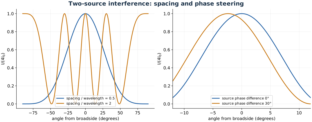
Two-source array factors show how spacing creates extra lobes and a relative phase steers them.
Problem 6.52 — locate a minimum from two in-phase radio sources
Paraphrased task. Locate a minimum from two in-phase radio sources.
Formula reference. Use (1), its definitions, and the topic illustration.
Worked application.
Put the two in-phase sources at \((\pm1.5,0)\) metres. Every point \((0,y)\) on their perpendicular bisector is at the same distance \(r=\sqrt{y^2+1.5^2}\) from both sources.
Therefore \(\Delta r=0\), \(\delta=2\pi\Delta r/\lambda=0\), and the interference factor is constructive everywhere on this line. There is no finite destructive fringe on the stated bisector; ordinary inverse-square falloff is not an interference minimum.
The printed \(2.25\,\mathrm m\) instead follows for a perpendicular line through one source: \(\sqrt{y^2+3^2}-y=\lambda/2=1.5\). Squaring gives \(9=3y+2.25\), hence \(y=2.25\,\mathrm m\). This is a different geometry, and unequal spherical-wave amplitudes also prevent exact cancellation there.
Result. As worded, no interference minimum exists on the perpendicular bisector. The printed 2.25 m belongs to a different path-difference construction.
Check. Always establish the two actual path lengths before substituting into a fringe condition.
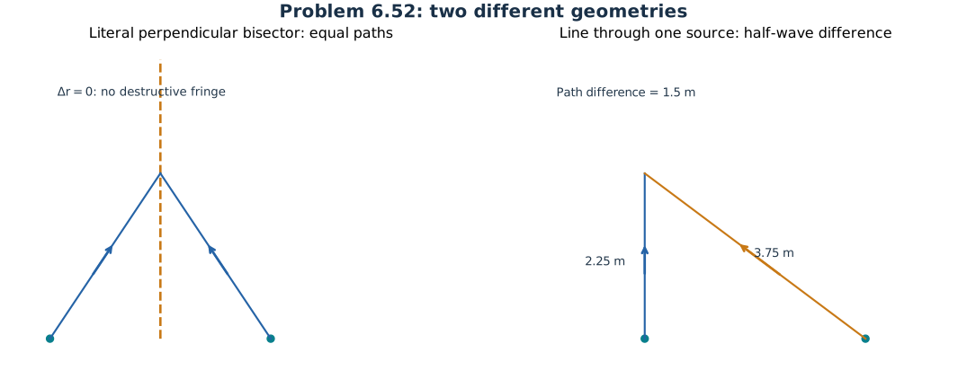
The literal perpendicular bisector has equal paths everywhere. The printed numerical endpoint instead uses a line through one source.
Problem 6.53 — identify when orthogonally polarized sources add without fringes
Paraphrased task. Identify when orthogonally polarized sources add without fringes.
Formula reference. Use (1), its definitions, and the topic illustration.
Worked application.
For coherent vector fields, time averaging gives \(I=I_1+I_2+2\sqrt{I_1I_2}(\hat{\mathbf e}_1\cdot\hat{\mathbf e}_2)\cos\delta\) for linear polarization unit vectors.
To make the interference term vanish everywhere, choose orthogonal polarization directions: \(\hat{\mathbf e}_1\cdot\hat{\mathbf e}_2=0\). Equal source phase alone does not guarantee equal phase at every point on the screen.
Then \(I=I_1+I_2\) regardless of path difference. At an individual screen point, a phase difference \(\delta=(m+1/2)\pi\) also makes the cross term zero, but that is a local condition rather than removal of the whole fringe pattern.
Result. Orthogonal linear polarizations remove the interference term throughout the screen.
Check. A following analyzer can project both beams onto a common polarization and restore interference.
Problem 6.54 — describe a two-source microwave radiation pattern
Paraphrased task. Describe a two-source microwave radiation pattern.
Formula reference. Use (1), its definitions, and the topic illustration.
Worked application.
The microwave wavelength is \(\lambda=c/\nu=0.30\,\mathrm m\). The source spacing is \(a=0.60\,\mathrm m=2\lambda\).
In the far field, \(\Delta r=a\sin\theta\), so \(I(\theta)=4I_0\cos^2(2\pi\sin\theta)\). Principal lobes satisfy \(a\sin\theta=m\lambda\), or \(\sin\theta=m/2\).
The allowed orders are \(m=-2,-1,0,1,2\). Over a complete angular section the maxima occur at \(0^\circ,30^\circ,90^\circ,150^\circ,180^\circ,210^\circ,270^\circ,330^\circ\). Minima satisfy \(\sin\theta=(2m+1)/4\) when the right side lies in \([-1,1]\).
Result. Eight lobe directions in a full plane, with pattern \(I/(4I_0)=\cos^2(2\pi\sin\theta)\).
Check. The pattern is symmetric under \(\theta\mapsto-\theta\) because the emitters have equal phase.
Problem 6.55 — verify spatially averaged energy conservation
Paraphrased task. Verify spatially averaged energy conservation.
Formula reference. Use (1), its definitions, and the topic illustration.
Worked application.
The coherent cross term is proportional to \(\cos(ka\cos\vartheta)\) if \(\vartheta\) is measured from the source-separation axis. For isotropic scalar emitters its spherical average is
\[\frac1{4\pi}\int\cos(ka\cos\vartheta)\,d\Omega =\frac12\int_{-1}^{1}\cos(ka\mu)\,d\mu =\frac{\sin(ka)}{ka}.\]When \(a\gg\lambda\), this average tends to zero: bright and dark angular regions nearly balance, leaving the incoherent-sum average. It is an asymptotic result, not exactly zero for every finite separation.
When \(a\ll\lambda\), the average tends to one. Equal in-phase fields behave approximately as a single doubled-amplitude source. Holding those field amplitudes fixed requires extra work from the mutually coupled sources; the enhanced radiated power does not violate energy conservation.
Result. The angularly averaged scalar cross term scales as \(\operatorname{sinc}(ka)\) and vanishes in the large-separation limit.
Check. One cannot simultaneously hold source amplitudes fixed and assume their required driving powers are unaffected by coherent coupling.
Problem 6.56 — include an intrinsic phase in the two-source pattern
Paraphrased task. Include an intrinsic phase in the two-source pattern.
Formula reference. Use (1), its definitions, and the topic illustration.
Worked application.
Define \(\Delta\epsilon=\epsilon_1-\epsilon_2\) and choose the path-sign convention \(\delta=ka\sin\theta+\Delta\epsilon\).
Equal individual irradiances give \(I=2I_0(1+\cos\delta)\).
Use \(1+\cos\delta=2\cos^2(\delta/2)\):
\[I(\theta)=4I_0\cos^2\left( \frac{\pi a\sin\theta}{\lambda}+\frac{\Delta\epsilon}{2}\right).\]Maxima obey \(ka\sin\theta+\Delta\epsilon=2\pi m\); a phase offset steers the lobe positions without moving the emitters.
Result. The phase offset translates the array factor in \(\sin\theta\), rather than rigidly rotating all lobes by the same angle.
Check. Setting \(\Delta\epsilon=0\) recovers the symmetric in-phase pattern.
Problem 6.57 — find lobe rotation caused by a thirty-degree phase shift
Paraphrased task. Find lobe rotation caused by a thirty-degree phase shift.
Formula reference. Use (1), its definitions, and the topic illustration.
Worked application.
Problem 6.54 has \(a/\lambda=2\), so \(ka=4\pi\). Introduce \(\Delta\epsilon=30^\circ=\pi/6\).
Track the formerly forward, zeroth-order maximum by setting \(4\pi\sin\theta+\pi/6=0\).
Hence \(\sin\theta=-1/24\) and \(\theta=-2.3880^\circ\). The displacement magnitude is about \(2^\circ23'\); reversing which emitter leads reverses the steering direction.
Result. The forward lobe shifts by \(2.39^\circ\) in magnitude.
Check. The required geometric path phase exactly cancels the imposed \(30^\circ\) source phase.
Problem 6.58 — choose phase shift for a twenty-degree lobe rotation
Paraphrased task. Choose phase shift for a twenty-degree lobe rotation.
Formula reference. Use (1), its definitions, and the topic illustration.
Worked application.
The referenced array has separation \(a=\lambda/2\), so \(ka=\pi\).
For a zeroth-order maximum at \(\theta_0=20^\circ\), enforce \(ka\sin\theta_0+\Delta\epsilon=0\).
Thus \(\Delta\epsilon=-\pi\sin20^\circ=-1.07449\,\mathrm{rad}=-61.5636^\circ\). Its magnitude is \(61.56^\circ\); the sign depends on the emitter labeling and desired side of broadside.
Result. A relative phase magnitude of \(61.56^\circ\) steers the central lobe by \(20^\circ\).
Check. Changing phase shifts the pattern in direction cosine, so other lobes do not necessarily move by exactly \(20^\circ\).
Wavefront-splitting interferometers
Formula and definitions.
In the paraxial limit the path difference is \(ay/L\), so successive orders differ by \(\lambda_0L/a\). Mirrors, biprisms, and split lenses first create two coherent virtual or real images; compute their effective separation and then reuse Young’s formula.
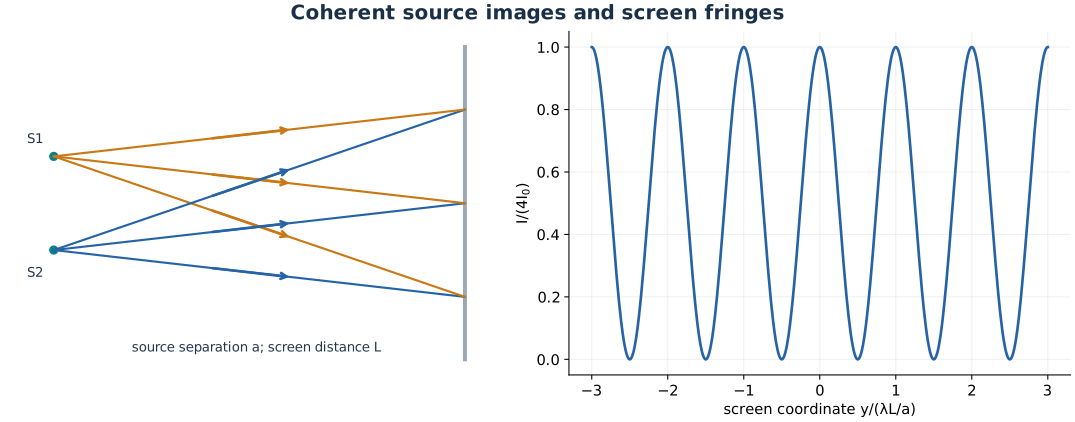
Two coherent source images produce alternating bright and dark screen positions according to their path difference.
Problem 6.59 — express Young-fringe spacing using source angular separation
Paraphrased task. Express young-fringe spacing using source angular separation.
Formula reference. Use (2), its definitions, and the topic illustration.
Worked application.
Near the central axis, sources separated by \(a\) at distance \(L\) subtend a small angle \(\beta\approx a/L\).
Moving along the screen by \(dy\) changes the path difference by \(d(\Delta r)\approx(a/L)dy=\beta\,dy\).
Consecutive like fringes require a path-difference increment of one wavelength: \(\beta\Delta y=\lambda_0\). Therefore \(\Delta y=\lambda_0/\beta\) for an air/vacuum observation region.
Result. \(\Delta y=\lambda_0/\beta\) in the paraxial limit, with \(\beta\) in radians.
Check. Greater apparent source separation makes the fringes closer together; in a medium use the wavelength in that medium.
Problem 6.60 — infer slit spacing from helium fringes
Paraphrased task. Infer slit spacing from helium fringes.
Formula reference. Use (2), its definitions, and the topic illustration.
Worked application.
Convert the wavelength: \(5875.618\,\text{\AA}=5.875618\times10^{-7}\,\mathrm m\). The screen distance is \(L=2.25\,\mathrm m\) and fringe spacing \(\Delta y=5.0\times10^{-4}\,\mathrm m\).
Rearrange Young’s spacing relation \(\Delta y=\lambda L/a\) to \(a=\lambda L/\Delta y\).
Substitution gives \(a=(5.875618\times10^{-7})(2.25)/(5.0\times10^{-4})=2.64403\times10^{-3}\,\mathrm m\).
Result. The slit separation is \(2.64\,\mathrm{mm}\).
Check. The angle \(a/L\approx1.18\times10^{-3}\) is small enough for the paraxial approximation.
Problem 6.61 — find virtual-source angular separation in a mirror geometry
Paraphrased task. Find virtual-source angular separation in a mirror geometry.
Formula reference. Use (2), its definitions, and the topic illustration.
Worked application.
For Fresnel’s double mirror, let the source be distance \(R\) from the mirrors’ intersection and the small mirror angle be \(\alpha\).
The two virtual source positions lie on a circle of radius \(R\), separated by angle \(2\alpha\); their separation is \(a=2R\sin\alpha\approx2R\alpha\).
A central screen point a distance \(d\) beyond the mirror intersection is approximately \(R+d\) from the virtual-source plane. The angular separation is therefore \(\beta\approx a/(R+d)=2R\alpha/(R+d)\).
Result. \(\beta\approx2R\alpha/(R+d)\) for small mirror tilt and paraxial observation.
Check. Do not confuse the mirror angle \(\alpha\) with the larger angular separation \(2\alpha\) of the virtual-source radius vectors.
Problem 6.62 — locate a Fresnel double-mirror fringe
Paraphrased task. Locate a fresnel double-mirror fringe.
Formula reference. Use (2), its definitions, and the topic illustration.
Worked application.
Convert the mirror angle to radians: \(\alpha=0.667\pi/180=0.0116411\). With \(R=0.1\,\mathrm m\), the virtual-source spacing is \(a\approx2R\alpha=0.00232827\,\mathrm m\).
The effective source-screen distance is \(L=R+d=1.1\,\mathrm m\). Thus \(\Delta y=\lambda L/a=(600\times10^{-9})(1.1)/0.00232827=0.283473\,\mathrm{mm}\).
The seventh bright fringe counted from the central maximum is \(y_7=7\Delta y=1.9843\,\mathrm{mm}\); the opposite side has \(y_{-7}=-y_7\).
Result. The seventh bright fringe is about \(1.98\,\mathrm{mm}\) from the axis.
Check. Use the source-to-screen distance \(R+d\), not just the mirror-to-screen distance \(d\).
Problem 6.63 — infer Fresnel-biprism angle from fringe spacing
Paraphrased task. Infer fresnel-biprism angle from fringe spacing.
Formula reference. Use (2), its definitions, and the topic illustration.
Worked application.
A thin biprism of small refracting angle \(\alpha\) deviates each half beam by \(\delta\approx(n-1)\alpha\).
With source distance \(R=1\,\mathrm m\), the virtual-source separation is \(a=2R(n-1)\alpha\). The screen is \(R+d=6\,\mathrm m\) from that virtual-source plane.
Solve \(\Delta y=\lambda(R+d)/[2R(n-1)\alpha]\):
\[\alpha=\frac{(500\times10^{-9})(6)}{2(1)(0.5)(0.6\times10^{-3})} =0.005\,\mathrm{rad}=0.28648^\circ.\]This value follows from the stated 1 m, 5 m, and 0.6 mm data; a different printed angle does not reproduce that spacing.
Result. Each small biprism angle is \(\alpha\approx0.286^\circ\) for the supplied distances.
Check. The resulting source separation is 5 mm, and \(500\,\mathrm{nm}\times6\,\mathrm m/5\,\mathrm{mm}=0.6\,\mathrm{mm}\).
Problem 6.64 — generalize biprism fringes to liquid immersion
Paraphrased task. Generalize biprism fringes to liquid immersion.
Formula reference. Use (2), its definitions, and the topic illustration.
Worked application.
For a prism of index \(n_g\) immersed in liquid \(n_l\), the small-angle Snell relation gives \(\delta\approx(n_g/n_l-1)\alpha\).
The two virtual sources are separated by \(a=2R\delta=2R(n_g-n_l)\alpha/n_l\). If the whole interference region is immersed, its wavelength is \(\lambda_l=\lambda_0/n_l\).
Substitute both changes, not just the new deviation:
\[\Delta y=\frac{\lambda_l(R+d)}a =\frac{\lambda_0(R+d)}{2R(n_g-n_l)\alpha}.\]If a formula is expressed using \(\lambda_l\) instead, its numerator is \(n_l\lambda_l(R+d)\). An extra \(n_l\) multiplying a vacuum wavelength would count the wavelength conversion incorrectly.
Result. For a fully immersed setup, \(\Delta y=\lambda_0(R+d)/[2R(n_g-n_l)\alpha]\).
Check. As the indices match, source splitting vanishes and fringe spacing diverges. A setup with liquid only around the prism requires its actual exit geometry.
Problem 6.65 — track Lloyd-mirror central fringe after inserting a plate
Paraphrased task. Track lloyd-mirror central fringe after inserting a plate.
Formula reference. Use (2), its definitions, and the topic illustration.
Worked application.
Replacing air by a plate of thickness \(t\) adds optical path \((n-1)t\) to the direct beam at near-normal incidence.
The Lloyd-mirror reflection already supplies a relative \(\pi\) phase. The zero-geometric-OPD dark fringe therefore moves until the original path imbalance cancels the plate’s added path; in the source geometry it moves upward.
Each fringe displacement represents an OPD change \(\lambda_0\), so the shift is \(N=(n-1)t/\lambda_0\) fringes. With broadband illumination the equal-total-OPD fringe is approximately achromatic, helping identify it among the coloured neighbouring fringes.
Result. The central dark fringe shifts upward by \((n-1)t/\lambda_0\) fringe spacings in the illustrated geometry.
Check. The direction depends on which beam receives the plate; insertion into the reflected arm would reverse it. Dispersion limits perfect white-light compensation.
Problem 6.66 — infer Lloyd source height from fringe spacing
Paraphrased task. Infer lloyd source height from fringe spacing.
Formula reference. Use (2), its definitions, and the topic illustration.
Worked application.
The mirror’s virtual source lies the same distance below the surface as the real source lies above it. If the source height is \(h\), their separation is \(a=2h\).
The fringe spacing is \(\Delta y=\lambda L/(2h)\), unaffected by the half-order shift caused by reflection.
Solve for height: \(h=(500\times10^{-9})(2)/[2(0.667\times10^{-3})]=7.4963\times10^{-4}\,\mathrm m\).
Result. The source is approximately \(0.750\,\mathrm{mm}\) above the reflecting surface.
Check. The reflection changes whether the central fringe is bright or dark, but not the separation of consecutive bright fringes.
Problem 6.67 — explain interference from a Billet split lens
Paraphrased task. Explain interference from a billet split lens.
Formula reference. Use (2), its definitions, and the topic illustration.
Worked application.
Each displaced half of the convex lens forms a real image of the same point source. For object and image distances \(s_o,s_i\), the common conjugate relation is \(1/f=1/s_o+1/s_i\).
A lens half displaced transversely by \(h\) images the on-axis object at \(y_i=h(1+s_i/s_o)\). Thus equal and opposite half displacements create two real image sources with a controlled separation.
After those foci the beams diverge and overlap. Because both came from the same source through symmetric paths, they interfere with \(I=I_1+I_2+2\sqrt{I_1I_2}\cos(2\pi\Delta r/\lambda)\). At a distant screen their fringe spacing is approximately \(\lambda L/a\).
Result. Billet’s split lens makes two coherent real image sources; fringes appear only where their outgoing beams overlap.
Check. Unlike the Fresnel biprism’s virtual sources, these intermediate image points are real foci traversed by the rays.
Amplitude splitting by thin films
Formula and definitions.
The round-trip optical thickness is \(2nd\cos\theta_t\). Add \(\pi\) for exactly one reflection from a higher-index boundary. A quarter-wave coating sets \(d=\lambda_0/(4n_c)\) and ideally \(n_c=\sqrt{n_0n_s}\). Newton-ring radii follow from \(d(r)\simeq r^2/(2R)\).
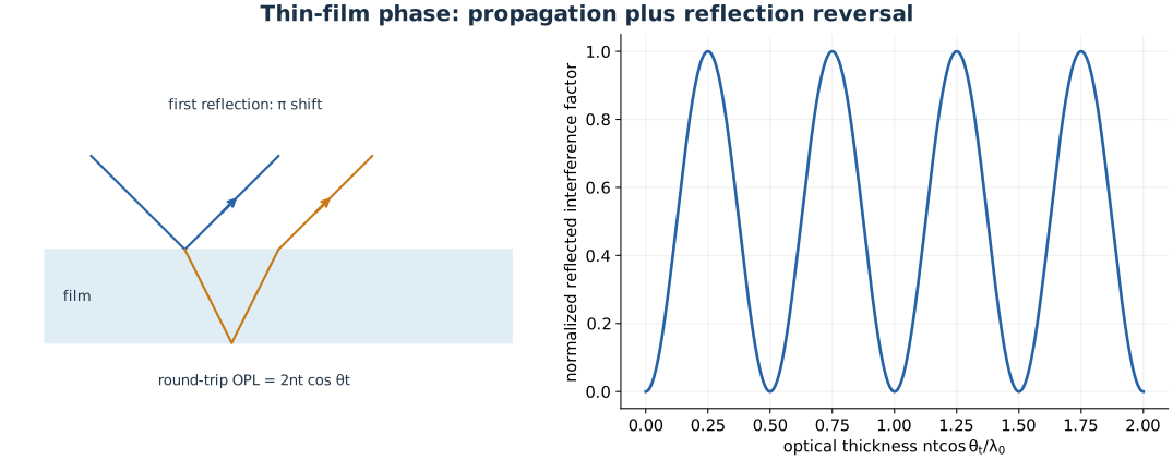
The thin-film round trip adds propagation phase; a single reflection reversal interchanges reflected maxima and minima.
Problem 6.68 — compute reflected-ray phase difference through a film
Paraphrased task. Compute reflected-ray phase difference through a film.
Formula reference. Use (3), its definitions, and the topic illustration.
Worked application.
The film thickness is \(t=0.002\,\mathrm{mm}=2000\,\mathrm{nm}\). Snell’s law gives \(\sin\theta_t=\sin30^\circ/1.5=1/3\), so \(\cos\theta_t=2\sqrt2/3\).
The round-trip optical path contributing to the reflected phase difference is \(2nt\cos\theta_t=5656.85\,\mathrm{nm}\); its propagation phase is \(4\pi nt\cos\theta_t/\lambda_0=22.6274\pi\).
Air-film reflection reverses phase while film-air reflection does not. Add one \(\pi\): \(\delta=23.6274\pi\), equivalent to \(1.6274\pi\) modulo \(2\pi\).
Result. The relative reflected phase is \(1.63\pi\) modulo \(2\pi\).
Check. Using \(2nt/\cos\theta_t\) alone misses the lateral wavefront compensation and gives an incorrect thin-film phase.
Problem 6.69 — derive equal-inclination extrema
Paraphrased task. Derive equal-inclination extrema.
Formula reference. Use (3), its definitions, and the topic illustration.
Worked application.
Let \(\lambda_f=\lambda_0/n_f\). For a film with exactly one reflected phase reversal, \(\delta=4\pi t\cos\theta_t/\lambda_f+\pi\).
A reflected maximum requires \(\delta=2\pi q\); therefore \(t\cos\theta_t=(2q-1)\lambda_f/4\). Relabel \(m=q-1\ge0\).
A minimum requires \(\delta=(2q+1)\pi\), giving \(t\cos\theta_t=q\lambda_f/2\). Thus maxima are at odd quarter-wave thicknesses and minima at integer half-wave thicknesses.
Result. Maxima: \(t\cos\theta_t=(2m+1)\lambda_f/4\); minima: \(t\cos\theta_t=2m\lambda_f/4\).
Check. With zero or two relative reflection reversals, the bright and dark conditions interchange.
Problem 6.70 — identify the central order of a parallel plate
Paraphrased task. Identify the central order of a parallel plate.
Formula reference. Use (3), its definitions, and the topic illustration.
Worked application.
The printed thickness is \(2.5\,\mathrm{mm}\); OCR can misread it as 2.6 mm. At the centre \(\theta_t=0\), with \(n=1.5\) and \(\lambda_0=750\,\mathrm{nm}\).
The round-trip order is \(m=2nt/\lambda_0=2(1.5)(2.5\times10^{-3})/(750\times10^{-9})=10000\).
This integer propagation order supplies \(2\pi m\); the additional single reflection reversal makes the reflected beams antiphase. The central fringe is therefore a reflected minimum.
Result. The central reflected fringe is a minimum of round-trip order \(10000\).
Check. At the same setting, transmission is maximal in an ideal lossless plate; bright/dark labels must specify the observed port.
Problem 6.71 — design an ideal single-layer antireflection coating
Paraphrased task. Design an ideal single-layer antireflection coating.
Formula reference. Use (3), its definitions, and the topic illustration.
Worked application.
A single quarter-wave layer must satisfy two independent conditions: opposite reflected phases and equal reflected amplitudes.
At normal incidence, amplitude matching between air \(n_0=1\) and substrate \(n_s=2.409\) gives \(n_f^2=n_0n_s\), hence \(n_f=\sqrt{2.409}=1.55210\).
The least positive odd-quarter-wave thickness is \(t=\lambda_0/(4n_f)=589/[4(1.55210)]=94.87\,\mathrm{nm}\). These choices make the net reflection vanish at the design wavelength for ideal real indices.
Result. Design index \(n_f\approx1.552\); thickness \(t\approx94.9\,\mathrm{nm}\).
Check. A quarter-wave thickness alone is not sufficient for zero reflectance unless the layer index also matches the geometric mean.
Problem 6.72 — choose magnesium-fluoride coating thickness
Paraphrased task. Choose magnesium-fluoride coating thickness.
Formula reference. Use (3), its definitions, and the topic illustration.
Worked application.
At near-normal incidence the destructive-reflection design uses an odd quarter-wave optical thickness: \(n_ft=(2m+1)\lambda_0/4\).
Choose \(m=0\) for the thinnest coating and use \(n_f=1.38\), \(\lambda_0=589\,\mathrm{nm}\).
This gives \(t=589/(4\cdot1.38)=106.703\,\mathrm{nm}\). It minimizes reflection at the design wavelength, but exact cancellation additionally requires an appropriate substrate index.
Result. The thinnest magnesium-fluoride layer is \(106.7\,\mathrm{nm}\).
Check. Its optical thickness is \(147.25\,\mathrm{nm}=589/4\), whereas its geometric thickness is smaller by \(n_f\).
Problem 6.73 — infer wedge angle from fringe spacing
Paraphrased task. Infer wedge angle from fringe spacing.
Formula reference. Use (3), its definitions, and the topic illustration.
Worked application.
For a small wedge angle \(\alpha\), film thickness grows as \(t(x)\approx\alpha x\).
Consecutive same-type reflected fringes differ in thickness by \(\Delta t=\lambda_0/(2n_f)\), so \(\Delta x=\lambda_0/(2n_f\alpha)\).
Substitute \(n_f=1.3290\), \(\lambda_0=589\,\mathrm{nm}\), \(\Delta x=0.2\,\mathrm{mm}\): \(\alpha=0.00110798\,\mathrm{rad}=0.06348^\circ\).
Result. The wedge angle is approximately \(0.0635^\circ\).
Check. The radian angle is much smaller than one, so \(\tan\alpha\approx\alpha\) is justified.
Problem 6.74 — locate the fourth wedge maximum and its film thickness
Paraphrased task. Locate the fourth wedge maximum and its film thickness.
Formula reference. Use (3), its definitions, and the topic illustration.
Worked application.
The apex is dark because the film has zero thickness and one relative reflection phase reversal. The first bright fringe is at \(t=\lambda_0/(4n_f)\).
Counting the fourth bright fringe from the apex gives the odd factor 7: \(t_4=7\lambda_0/(4n_f)=7(589)/(4\cdot1.3290)=775.58\,\mathrm{nm}\).
Bright positions are halfway between consecutive dark positions. With \(\Delta x=0.2\,\mathrm{mm}\), \(x_4=(4-1/2)\Delta x=0.700\,\mathrm{mm}\); equivalently \(x_4=t_4/\alpha\).
Result. The fourth maximum occurs at thickness \(7.76\times10^{-7}\,\mathrm m\), \(0.700\,\mathrm{mm}\) from the apex.
Check. Counting the first bright fringe as order zero prevents an off-by-one half-wave error.
Problem 6.75 — infer liquid index from Newton-ring diameters
Paraphrased task. Infer liquid index from newton-ring diameters.
Formula reference. Use (3), its definitions, and the topic illustration.
Worked application.
At fixed bright-ring order and lens curvature, Newton’s ring equation has \(r_m^2\propto1/n\); the same scaling holds for squared diameter.
Divide the before/after equations to remove wavelength, curvature, and order: \(n_{\rm liquid}/n_{\rm air}=D_{\rm air}^2/D_{\rm liquid}^2\).
With \(D_{\rm air}=2.52\,\mathrm{cm}\), \(D_{\rm liquid}=2.21\,\mathrm{cm}\), and \(n_{\rm air}\approx1\), \(n=(2.52/2.21)^2=1.30023\).
Result. The liquid index is approximately \(1.30\).
Check. A liquid with index greater than air shrinks the rings, matching the observed diameter decrease.
Problem 6.76 — recover lens curvature from separated Newton-ring orders
Paraphrased task. Recover lens curvature from separated newton-ring orders.
Formula reference. Use (3), its definitions, and the topic illustration.
Worked application.
Allow an unknown central film gap \(t_0\), since the centre is bright rather than the usual contact dark. The gap profile is \(t(r)=t_0+r^2/(2R)\).
Subtract the dark-ring conditions at orders 85 and 5. The unknown \(t_0\) and any common order offset cancel, giving \(r_{85}^2-r_5^2=80\lambda R\) for an air gap.
Therefore \(R=[(0.01871)^2-(0.01414)^2]/[80(550\times10^{-9})]=3.411\,\mathrm m\).
Result. The convex lens radius is approximately \(3.41\,\mathrm m\).
Check. Using radius-squared differences avoids assuming perfect contact or assigning an absolute order to the bright centre.
Problem 6.77 — generalize Newton rings to two curved surfaces
Paraphrased task. Generalize newton rings to two curved surfaces.
Formula reference. Use (3), its definitions, and the topic illustration.
Worked application.
The opposing spherical sags are approximately \(r^2/(2R_1)\) and \(r^2/(2R_2)\). With \(R_2>R_1\), the air gap is \(t(r)=\tfrac12r^2(1/R_1-1/R_2)\).
Reflected dark rings with one phase reversal satisfy \(2t=m\lambda_0\).
Substitute the sag difference and solve:
\[r_m=\sqrt{\frac{m\lambda_0}{1/R_1-1/R_2}} =\sqrt{\frac{m\lambda_0R_1R_2}{R_2-R_1}}.\]
Result. \(r_m=\sqrt{m\lambda_0R_1R_2/(R_2-R_1)}\) for a contacting air film.
Check. Letting \(R_2\to\infty\) recovers the standard plano-convex Newton-ring result \(r_m^2=m\lambda_0R_1\).
Amplitude-splitting interferometers
Formula and definitions.
A mirror displacement changes a Michelson round trip by twice the mechanical travel. For a doublet, visibility goes from maximum to minimum when the two wavelengths acquire a relative phase of \(\pi\). A gas cell adds optical path \((n-1)L\) per traversed cell length.
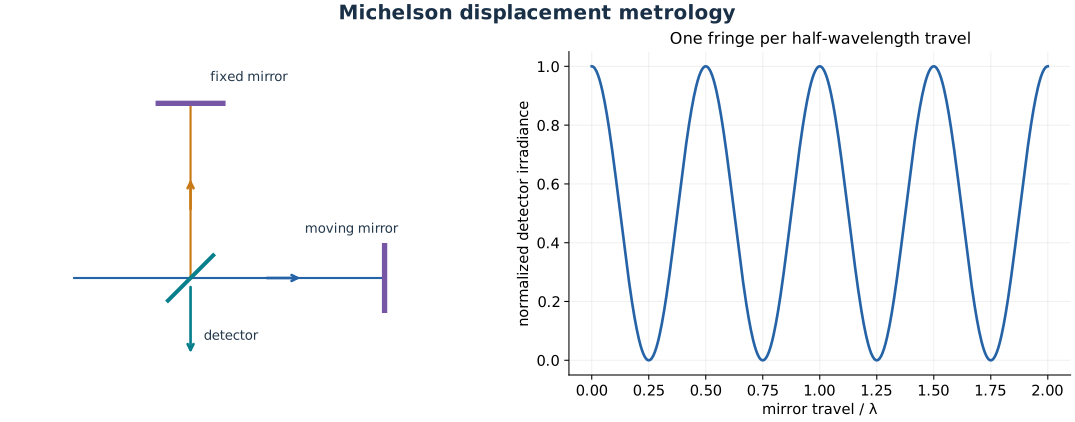
A Michelson mirror displacement changes optical path twice as much, explaining the factor of two in fringe counting.
Problem 6.78 — prove Michelson equal-inclination rings collapse as arms equalize
Paraphrased task. Prove michelson equal-inclination rings collapse as arms equalize.
Formula reference. Use (4), its definitions, and the topic illustration.
Worked application.
Follow a fixed Michelson ring order \(m\) satisfying \(2d\cos\theta_m=m\lambda_0\), where \(d\) is the arm-length difference.
Solve \(\cos\theta_m=m\lambda_0/(2d)\). As positive \(d\) decreases, the right side increases, so \(\theta_m\) decreases and the ring radius shrinks.
The ring reaches the axis at \(d=m\lambda_0/2\), where \(\theta_m=0\). For smaller \(d\), the same order has no real angle and disappears; successive orders collapse in turn as equal arms are approached.
Result. Each fixed-order ring contracts to the centre and disappears as its allowed arm difference is crossed.
Check. A given nonzero order reaches the centre before \(d=0\); it cannot be followed continuously all the way to equal arms.
Problem 6.79 — find sodium-doublet mirror travel from visibility maximum to minimum
Paraphrased task. Find sodium-doublet mirror travel from visibility maximum to minimum.
Formula reference. Use (4), its definitions, and the topic illustration.
Worked application.
The two vacuum wavelengths are \(\lambda_1=589.5923\,\mathrm{nm}\) and \(\lambda_2=588.9953\,\mathrm{nm}\), separated by \(0.5970\,\mathrm{nm}\).
For mirror displacement \(x\), the OPD changes by \(2x\). The phase difference between the two fringe systems changes by \(4\pi x(1/\lambda_2-1/\lambda_1)\).
A visibility maximum becomes a minimum when this phase difference reaches \(\pi\). Hence \(x=\lambda_1\lambda_2/[4(\lambda_1-\lambda_2)]\approx0.14542\,\mathrm{mm}\).
Result. Move the mirror approximately \(0.1454\,\mathrm{mm}\) from maximum to minimum visibility.
Check. Maximum-to-maximum travel is twice as large; the optical-path change is itself twice the mirror travel.
Problem 6.80 — find Michelson mirror travel for ten thousand fringes
Paraphrased task. Find michelson mirror travel for ten thousand fringes.
Formula reference. Use (4), its definitions, and the topic illustration.
Worked application.
Moving one Michelson mirror through \(x\) changes the round-trip optical path by \(2x\).
Each passing bright fringe represents one wavelength of OPD, so \(N=2x/\lambda_0\) and \(x=N\lambda_0/2\).
With \(N=10000\) and \(\lambda_0=605.7802105\,\mathrm{nm}\), \(x=3028901.0525\,\mathrm{nm}=3.028901\,\mathrm{mm}\).
Result. The mirror must travel \(3.0289\,\mathrm{mm}\).
Check. A result twice as large would forget that the beam traverses the moving arm twice.
Problem 6.81 — derive the small-angle radius of a Michelson dark ring
Paraphrased task. Derive the small-angle radius of a michelson dark ring.
Formula reference. Use (4), its definitions, and the topic illustration.
Worked application.
A dark centre has some axial order \(m_0=2d/\lambda_0\). At increasing angle the order decreases, so the \(p`th surrounding dark ring has :math:`m=m_0-p\).
Subtract \(2d\cos\theta_p=(m_0-p)\lambda_0\) from the axial equation \(2d=m_0\lambda_0\) to obtain \(2d(1-\cos\theta_p)=p\lambda_0\).
For small angle, \(1-\cos\theta_p\approx\theta_p^2/2\); hence \(\theta_p\approx\sqrt{p\lambda_0/d}\).
Result. Exact: \(\cos\theta_p=1-p\lambda_0/(2d)\); paraxial: \(\theta_p\approx\sqrt{p\lambda_0/d}\).
Check. Ring number counted outward is not the same as absolute interference order; the latter decreases outward.
Problem 6.82 — calculate the fifteenth dark-ring angle
Paraphrased task. Calculate the fifteenth dark-ring angle.
Formula reference. Use (4), its definitions, and the topic illustration.
Worked application.
Use \(p=15\), \(d=1\,\mathrm{cm}=0.01\,\mathrm m\), and \(\lambda_0=400\,\mathrm{nm}\).
The small-angle expression gives \(\theta_{15}=\sqrt{15(400\times10^{-9})/0.01}=0.0244949\,\mathrm{rad}\).
Converting to degrees gives \(1.40345^\circ\approx1^\circ24'\). The exact expression \(\arccos[1-15\lambda_0/(2d)]\) changes this only slightly.
Result. The fifteenth dark ring subtends a half-angle of about \(1.40^\circ\).
Check. This is the angular radius of the ring; its full angular diameter is twice this value.
Problem 6.83 — infer gas index with a Jamin interferometer
Paraphrased task. Infer gas index with a jamin interferometer.
Formula reference. Use (4), its definitions, and the topic illustration.
Worked application.
In the Jamin arrangement the test cell is traversed once. Replacing vacuum by gas adds OPD \((n-1)L\), where \(L=0.35\,\mathrm m\).
The 75 observed fringe passages imply \((n-1)L=75\lambda_0\).
Thus \(n=1+75(650\times10^{-9})/0.35=1.000139286\).
Result. The gas refractive index is \(n\approx1.000139\).
Check. Do not import the Michelson factor of two into this single-pass cell measurement.
Problem 6.84 — explain and apply a Mach-Zehnder interferometer
Paraphrased task. Explain and apply a mach-zehnder interferometer.
Formula reference. Use (4), its definitions, and the topic illustration.
Worked application.
The first beam splitter divides the incident field into two spatially separated arms. Each arm reflects from its own mirror, and the second beam splitter overlaps their fields.
Their relative phase is \(\delta(x,y)=2\pi\,\mathrm{OPD}(x,y)/\lambda+\delta_{\rm BS}\). At either output the irradiance has the form \(I_1+I_2+2\sqrt{I_1I_2}\cos\delta\); the other output is complementary for a balanced lossless system.
A slight relative mirror tilt adds an approximately linear phase ramp, producing straight carrier fringes. A specimen in one arm changes \(\mathrm{OPD}=\int(n-n_{\rm ref})\,ds\); fringe shifts then map refractive-index variations, for example in gas flows or a wind tunnel.
Result. The Mach–Zehnder is a two-arm, single-pass amplitude-splitting interferometer, closely related in measurement purpose to the Jamin arrangement.
Check. Both path matching within the coherence length and spatial/polarization overlap at the second splitter are needed for visible fringes.
Coherence
Formula and definitions.
Convert fractional stability \(\Delta\nu/\nu\) to an absolute linewidth using \(\nu=c/\lambda_0\). The reciprocal linewidth is the coherence time and multiplication by \(c\) gives coherence length. For a stellar disk, the first visibility zero supplies its angular diameter.
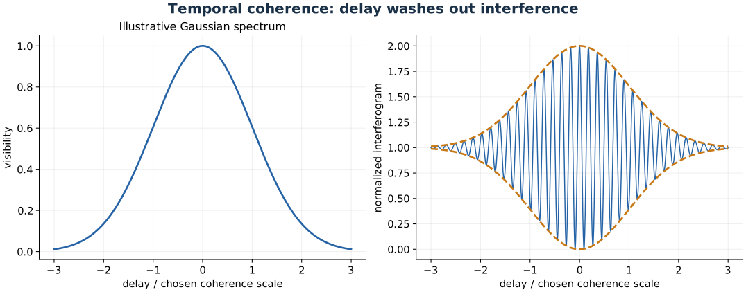
Finite spectral width limits fringe visibility as optical delay grows. The plotted Gaussian envelope is illustrative, not a universal line shape.
Problem 6.85 — infer coherence time and length from laser frequency stability
Paraphrased task. Infer coherence time and length from laser frequency stability.
Formula reference. Use (5), its definitions, and the topic illustration.
Worked application.
At \(\lambda=1153\,\mathrm{nm}\), the optical frequency is \(\nu=c/\lambda\approx2.60\times10^{14}\,\mathrm{Hz}\).
In the source’s estimate, identify the quoted fractional frequency spread \(s=8\times10^{-14}\) with \(\Delta\nu/\nu\). This gives \(\Delta\nu=s\nu\approx20.8\,\mathrm{Hz}\).
Using the order-of-magnitude convention \(\tau_c\sim1/\Delta\nu\), obtain \(\tau_c\approx0.0480\,\mathrm s\) and \(L_c=c\tau_c\approx1.44\times10^7\,\mathrm m\).
Result. The wave-train estimate is \(\tau_c\approx4.8\times10^{-2}\,\mathrm s\), \(L_c\approx14.4\,\mathrm{Mm}\).
Check. A measured frequency-stability statistic is not automatically a spectral linewidth; rigorous coherence requires the frequency-noise spectrum and a specified linewidth/coherence convention.
Problem 6.86 — estimate linewidth and coherence length from transition time
Paraphrased task. Estimate linewidth and coherence length from transition time.
Formula reference. Use (5), its definitions, and the topic illustration.
Worked application.
For a wave train of duration \(\tau=10^{-8}\,\mathrm s\), estimate \(\Delta\nu\sim1/\tau=10^8\,\mathrm{Hz}\).
Differentiate \(\nu=c/\lambda\) in magnitude: \(\Delta\lambda\approx\lambda^2\Delta\nu/c\). With \(\lambda=650\,\mathrm{nm}\), \(\Delta\lambda\approx1.41\times10^{-13}\,\mathrm m=1.41\times10^{-4}\,\mathrm{nm}\).
The coherence length in this convention is \(L_c=c\tau\approx3.0\,\mathrm m\).
Result. Approximate linewidth \(10^8\,\mathrm{Hz}\) or \(1.41\times10^{-4}\,\mathrm{nm}\); coherence length \(3\,\mathrm m\).
Check. Numerical factors such as \(\pi\) depend on the assumed line shape and the exact definition of coherence time; these are wave-train estimates.
Problem 6.87 — infer filter linewidth and Michelson range from wave-train length
Paraphrased task. Infer filter linewidth and michelson range from wave-train length.
Formula reference. Use (5), its definitions, and the topic illustration.
Worked application.
A train of 50 wavelengths has \(L_c=50\lambda=50(650\,\mathrm{nm})=32.5\,\mathrm{\mu m}\).
From \(L_c\sim\lambda^2/\Delta\lambda\), the filter bandwidth is \(\Delta\lambda\sim\lambda/50=13\,\mathrm{nm}\).
In a Michelson interferometer, mirror displacement \(x\) introduces \(2x\) OPD. Starting at matched paths, appreciable overlap is lost on the scale \(x\sim L_c/2=16.25\,\mathrm{\mu m}=0.01625\,\mathrm{mm}\).
Result. Bandwidth about \(13\,\mathrm{nm}\); one-sided mirror travel from equal paths about \(16.25\,\mathrm{\mu m}\).
Check. This is a coherence scale, not a sharp universal visibility cutoff for every filter profile.
Problem 6.88 — relate inverse fractional stability to wavelengths per wave train
Paraphrased task. Relate inverse fractional stability to wavelengths per wave train.
Formula reference. Use (5), its definitions, and the topic illustration.
Worked application.
The number of optical cycles in a train is \(N=\nu\tau_c\), equivalently \(N=L_c/\lambda\).
Use the bandwidth estimate \(\tau_c\sim1/\Delta\nu\), giving \(N\sim\nu/\Delta\nu\).
If the fractional spectral width is \(s=\Delta\nu/\nu\), then \(N\sim1/s\). A fractional width of \(10^{-6}\), for example, corresponds to roughly a million optical cycles per train in this model.
Result. \(N\sim(\Delta\nu/\nu)^{-1}\).
Check. This statement concerns a spectral-width interpretation of stability; drift and short-term noise measures need not equal that width.
Problem 6.89 — find coherence length and cycle count through a narrow filter
Paraphrased task. Find coherence length and cycle count through a narrow filter.
Formula reference. Use (5), its definitions, and the topic illustration.
Worked application.
The filter has central wavelength \(\lambda=550\,\mathrm{nm}\) and narrow passband \(\Delta\lambda=1.5\,\mathrm{nm}\).
Compute \(L_c\sim\lambda^2/\Delta\lambda=550^2/1.5\,\mathrm{nm}=201666.7\,\mathrm{nm}=2.0167\times10^{-4}\,\mathrm m\).
The number of wavelengths is \(N=L_c/\lambda=550/1.5=366.67\).
Result. Coherence length approximately \(0.202\,\mathrm{mm}\), containing about 367 wavelengths.
Check. \(\Delta\lambda/\lambda\approx0.0027\ll1\), so the narrowband frequency-to-wavelength conversion is valid.
Problem 6.90 — infer stellar angular diameter with a Michelson interferometer
Paraphrased task. Infer stellar angular diameter with a michelson interferometer.
Formula reference. Use (5), its definitions, and the topic illustration.
Worked application.
Model the star as a uniformly bright circular disk of angular diameter \(\phi\). Its two-aperture visibility is \(V=|2J_1(\pi h\phi/\lambda)/(\pi h\phi/\lambda)|\).
The first zero of \(J_1\) is 3.8317, so the first vanished-fringe baseline obeys \(h_0\phi/\lambda=3.8317/\pi=1.21967\).
Convert \(h_0=121\,\mathrm{in}=3.0734\,\mathrm m\), then \(\phi=1.21967(570\times10^{-9})/3.0734=2.262\times10^{-7}\,\mathrm{rad}\). This is \(1.296\times10^{-5}\,\mathrm{deg}\) or \(0.0467\) arcsec.
Result. Uniform-disk angular diameter \(\phi\approx2.26\times10^{-7}\,\mathrm{rad}=0.0467\) arcsec.
Check. The factor 1.22 depends on a circular uniform-disk brightness model; limb darkening changes the inferred physical diameter.
Problem 6.91 — compare methane-stabilized laser coherence over a decade
Paraphrased task. Compare methane-stabilized laser coherence over a decade.
Formula reference. Use (5), its definitions, and the topic illustration.
Worked application.
Keep the wavelength 1153 nm, hence \(\nu\approx2.60\times10^{14}\,\mathrm{Hz}\). Interpret the new \(6\times10^{-16}\) fractional spread with the same heuristic as Problem 6.85.
The estimated width is \(\Delta\nu\approx0.156\,\mathrm{Hz}\), giving \(\tau_c\sim1/\Delta\nu\approx6.41\,\mathrm s\).
The ratio of inferred coherence times is the inverse ratio of fractional spreads: \(\tau_{1973}/\tau_{1963}=(8\times10^{-14})/(6\times10^{-16})=133.3\). The quoted 100 s stability interval is the observation interval, not itself the coherence time.
Result. The source’s estimate increases from about \(0.048\,\mathrm s\) to \(6.4\,\mathrm s\), a factor of 133.
Check. This historical comparison assumes the quoted stability values represent comparable spectral widths; it is not a general conversion rule for laser stability specifications.