Chapter 2: Electromagnetic Waves and Photons

Source: Eugene Hecht, Schaum’s Outline of Theory and Problems of Optics (1975), Chapter 2. The entries below cover only the chapter’s Supplementary Problems; prompts are paraphrased and are not reproduced.

Each numbered solution states its assumptions, develops the algebra, substitutes the relevant data, and checks the result. Original SVG illustrations show the ray geometry, field relationships, or calculated curves. Diagrams are schematic unless their axes specify a scale. Source inconsistencies and approximations are identified explicitly rather than silently copied into the answer.

Maxwell equations and electromagnetic waves

Formula and definitions.

(1)\[\mathbf B=\frac{1}{v}\hat{\mathbf k}\times\mathbf E,\qquad \mathbf E=-v\hat{\mathbf k}\times\mathbf B,\qquad v=\frac{c}{n}\]

For a transverse plane wave, \(\mathbf E\), \(\mathbf B\), and \(\hat{\mathbf k}\) form a right-handed orthogonal triad. Their amplitudes satisfy \(E_0=vB_0\); the phase and propagation argument are common to both fields.

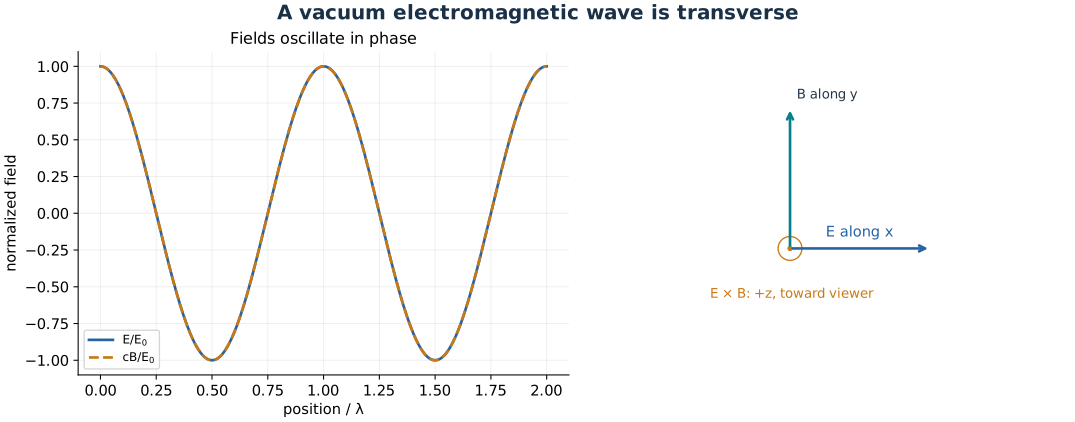
Electric field, magnetic field, and propagation direction are mutually perpendicular in a vacuum plane wave.

Problem 2.26 — reconstruct E from a specified plane-wave B field

Paraphrased task. Reconstruct e from a specified plane-wave b field.

Formula reference. Use (1), its definitions, and the topic illustration.

Worked application.

1. Read \(k=4\pi10^6\,\mathrm{rad/m}\) and \(B_0=66.7\times10^{-8}\,\mathrm T\). The argument \(k(z-ct)\) gives propagation along \(+z\).

2. The field relation is \(\mathbf E=-c\hat{\mathbf z}\times\mathbf B\). Because \(\hat{\mathbf z}\times\hat{\mathbf y}=-\hat{\mathbf x}\), the electric field points along \(+x\).

3. Calculate \(E_0=cB_0\simeq200\,\mathrm{V/m}\) and \(\lambda=2\pi/k=5.00\times10^{-7}\,\mathrm m\). Both fields have the same phase.

Result. \(\mathbf E=200\hat{\mathbf x}\sin[4\pi10^6(z-3\times10^8t)]\,\mathrm{V/m}\); \(\lambda=500\,\mathrm{nm}\) and \(v=c\).

Check. \(\hat{\mathbf x}\times\hat{\mathbf y}=\hat{\mathbf z}\) confirms the Poynting-vector direction.

Problem 2.27 — reconstruct B from a graphed electric field

Paraphrased task. Reconstruct b from a graphed electric field.

Formula reference. Use (1), its definitions, and the topic illustration.

Worked application.

1. The electric-field snapshot has a 20 V/m peak, a 1 mm spatial period, and a positive crest at the origin. Therefore use \(E_y=20\cos[k(x-ct)]\) with \(k=2\pi\times10^3\,\mathrm{rad/m}\).

2. Divide the electric amplitude by \(c\): \(B_0=20/(3\times10^8)=6.67\times10^{-8}\,\mathrm T\).

3. The wave moves along \(+x\), so \(\mathbf B=(1/c)\hat{\mathbf x}\times\mathbf E\) points along \(+z\). The same cosine phase is required for positive forward energy flow.

Result. \(B_z=6.67\times10^{-8}\cos[2\pi10^3(x-3\times10^8t)]\,\mathrm T\); \(B_x=B_y=0\).

Check. A 1 mm separation reproduces the snapshot; the time period is \(\lambda/c=3.33\times10^{-12}\,\mathrm s\).

Problem 2.28 — reconstruct E from a graphed magnetic field

Paraphrased task. Reconstruct e from a graphed magnetic field.

Formula reference. Use (1), its definitions, and the topic illustration.

Worked application.

1. Read the graph’s axes before converting: \(B_0=2\times10^{-6}\,\mathrm T\) and \(T=10^{-14}\,\mathrm s\). The initial value is a positive crest.

2. Hence \(E_0=cB_0=600\,\mathrm{V/m}\), \(\lambda=cT=3\times10^{-6}\,\mathrm m\), and \(k=(2\pi/3)10^6\,\mathrm{rad/m}\).

3. For positive-x propagation with \(\mathbf B\parallel+z\), \(\mathbf E=-c\hat{\mathbf x}\times\mathbf B\parallel+y\). Use a cosine with the measured period.

Result. \(\mathbf E=600\hat{\mathbf y}\cos[(2\pi/3)10^6(x-3\times10^8t)]\,\mathrm{V/m}\).

Check. The earlier 7600 V/m value does not follow the graph; 600 V/m gives the measured 2 microtesla amplitude.

Problem 2.29 — determine a field from wavelength, direction, and irradiance

Paraphrased task. Determine a field from wavelength, direction, and irradiance.

Formula reference. Use (1), its definitions, and the topic illustration.

Worked application.

1. In vacuum, invert the time-averaged flux formula:

   \[E_0=\sqrt{\frac{2I}{c\epsilon_0}} =\sqrt{\frac{2(1.197)}{(3.00\times10^8)(8.854\times10^{-12})}} \simeq30.0\,\mathrm{V/m}.\]

2. Transversality removes the y component of \(\mathbf B\). Since it lies in the xy plane, choose it along \(+x\); positive-y energy flow then requires \(\mathbf E\parallel+z\).

3. With \(\lambda=500\,\mathrm{nm}\), \(k=4\pi10^6\,\mathrm{rad/m}\). The initial phase is unspecified, so zero is an admissible choice.

Result. \(\mathbf E=30\hat{\mathbf z}\sin[4\pi10^6(y-ct)]\,\mathrm{V/m}\) is one valid field.

Check. \(\hat{\mathbf z}\times\hat{\mathbf x}=\hat{\mathbf y}\); a simultaneous reversal of both transverse fields is equally valid.

Index of refraction

Formula and definitions.

(2)\[v=\frac{c}{n},\qquad \lambda=\frac{\lambda_0}{n},\qquad k=\frac{2\pi n}{\lambda_0},\qquad \Delta t=\frac{L(n_2-n_1)}{c}\]

Frequency is unchanged at a stationary interface, so reducing the phase velocity by \(n\) reduces wavelength by the same factor. For a nonmagnetic transparent material, \(n\simeq\sqrt{\epsilon_r}\).

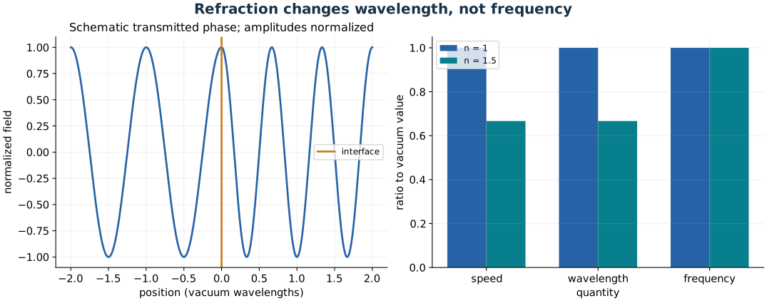
An interface preserves frequency while changing speed and wavelength. The example compares indices 1 and 1.5.

Problem 2.30 — compute propagation number in a dielectric

Paraphrased task. Compute propagation number in a dielectric.

Formula reference. Use (2), its definitions, and the topic illustration.

Worked application.

1. Keep the given 600 nm as the vacuum wavelength \(\lambda_0\); the frequency stays constant at the interface.

2. The material wavelength is \(\lambda=\lambda_0/n=600/1.5=400\,\mathrm{nm}\).

3. Therefore \(k=2\pi/\lambda=2\pi/(400\times10^{-9})=1.571\times10^7\,\mathrm{rad/m}\). The equivalent single substitution is \(k=2\pi n/\lambda_0\).

Result. \(k=1.57\times10^7\,\mathrm{rad/m}\).

Check. The propagation number increases by the factor \(n\), while the wavelength decreases by that factor.

Problem 2.31 — infer path length from a transit-time difference

Paraphrased task. Infer path length from a transit-time difference.

Formula reference. Use (2), its definitions, and the topic illustration.

Worked application.

1. The equal geometric path lengths give \(t_{\rm liquid}=1.46L/c\) and \(t_{\rm air}=L/c\).

2. Subtract before solving: \(\Delta t=(1.46-1)L/c\). The required delay is \(10^{-6}\,\mathrm s\).

3. Consequently \(L=c\Delta t/0.46=(3.00\times10^8)(10^{-6})/0.46=652\,\mathrm m\).

Result. A path length of approximately \(6.52\times10^2\,\mathrm m\) is required.

Check. At this length the transit times are approximately 3.17 and 2.17 microseconds, differing by one microsecond.

Problem 2.32 — compare wavelengths in diamond and zircon

Paraphrased task. Compare wavelengths in diamond and zircon.

Formula reference. Use (2), its definitions, and the topic illustration.

Worked application.

1. For each medium use the same vacuum wavelength: \(\lambda_D=589/2.417=243.7\,\mathrm{nm}\) and \(\lambda_Z=589/1.923=306.3\,\mathrm{nm}\).

2. Divide the two equations so the common vacuum wavelength cancels:

   \[\frac{\lambda_D}{\lambda_Z}=\frac{n_Z}{n_D} =\frac{1.923}{2.417}=0.7956.\]

3. The ratio is less than one because diamond has the larger index, not because the frequency changes.

Result. \(\lambda_D/\lambda_Z\simeq0.796\).

Check. The reciprocal index ordering is essential; taking \(n_D/n_Z\) predicts the wrong wavelength ordering.

Problem 2.33 — infer refractive index from dielectric constant

Paraphrased task. Infer refractive index from dielectric constant.

Formula reference. Use (2), its definitions, and the topic illustration.

Worked application.

1. Maxwell’s wave speed gives \(v=1/\sqrt{\mu\epsilon}\). Dividing vacuum speed by this speed yields \(n=\sqrt{\mu_r\epsilon_r}\).

2. For a nonmagnetic transparent dielectric, take \(\mu_r\simeq1\) and the specified dielectric constant \(\epsilon_r=2.381\).

3. Thus \(n=\sqrt{2.381}=1.5431\). This identification assumes the dielectric constant is appropriate to the optical frequency; a static value need not be interchangeable in a dispersive material.

Result. \(n\simeq1.543\) under the nonmagnetic, optical-frequency assumption.

Check. Squaring the calculated index recovers 2.381.

Irradiance

Formula and definitions.

(3)\[I=\frac{P}{A},\qquad U=IAt,\qquad \langle S\rangle=I=\frac12 c\epsilon_0E_0^2,\qquad P_{\rm iso}=4\pi r^2I\]

The instantaneous Poynting vector is \(\mathbf S=\mathbf E\times\mathbf H\). Since \(\langle\sin^2\Phi\rangle=1/2\) and \(H_0=E_0/Z_0\), its cycle average becomes \(I=E_0^2/(2Z_0)=c\epsilon_0E_0^2/2\).

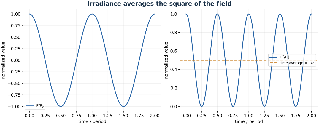
Irradiance follows the time average of the squared field, not the average field itself.

Problem 2.34 — convert flux density and exposure time to energy

Paraphrased task. Convert flux density and exposure time to energy.

Formula reference. Use (3), its definitions, and the topic illustration.

Worked application.

1. The beam strikes normally and is perfectly absorbed, so the deposited power is irradiance times illuminated area.

2. Keeping the supplied centimetre units consistent gives \(P=(10\,\mathrm{W/cm^2})(1\,\mathrm{cm^2})=10\,\mathrm W\).

3. Multiply by exposure time: \(U=Pt=(10)(1000)=10^4\,\mathrm J\). In SI, the equivalent irradiance and area are \(10^5\,\mathrm{W/m^2}\) and \(10^{-4}\,\mathrm{m^2}\).

Result. \(U=10^4\,\mathrm J\).

Check. Watts times seconds are joules; no factor of \(c\) is needed for an energy calculation.

Problem 2.35 — obtain focused-laser irradiance and field amplitude

Paraphrased task. Obtain focused-laser irradiance and field amplitude.

Formula reference. Use (3), its definitions, and the topic illustration.

Worked application.

1. Convert \(P=3\,\mathrm{kW}=3000\,\mathrm W\) and \(A=10^{-5}\,\mathrm{cm^2}=10^{-9}\,\mathrm{m^2}\).

2. The irradiance is \(I=P/A=3.00\times10^{12}\,\mathrm{W/m^2}\).

3. Recover the peak, not RMS, electric field:

   \[E_0=\sqrt{\frac{2I}{c\epsilon_0}} =\sqrt{\frac{6.00\times10^{12}}{2.656\times10^{-3}}} =4.75\times10^7\,\mathrm{V/m}.\]

   The quoted wavelength and cutting time provide context but are unnecessary for this amplitude calculation.

Result. \(I=3.00\times10^{12}\,\mathrm{W/m^2}\), \(E_0\simeq4.75\times10^7\,\mathrm{V/m}\).

Check. The area conversion uses \(1\,\mathrm{cm^2}=10^{-4}\,\mathrm{m^2}\), not \(10^{-2}\).

Problem 2.36 — derive the vacuum irradiance coefficient

Paraphrased task. Derive the vacuum irradiance coefficient.

Formula reference. Use (3), its definitions, and the topic illustration.

Worked application.

1. The peak magnetic field in vacuum is \(B_0=E_0/c\), so the instantaneous Poynting flux is \(S=E_0^2\cos^2\Phi/(\mu_0c)\).

2. Average over a complete cycle: \(\langle\cos^2\Phi\rangle=1/2\). Since \(1/(\mu_0c)=c\epsilon_0\), obtain \(I=c\epsilon_0E_0^2/2\).

3. Substitute constants: \(c\epsilon_0/2=(2.998\times10^8)(8.854\times10^{-12})/2=1.327\times10^{-3}\) in SI.

Result. \(I=(1.33\times10^{-3}\,\mathrm{W/V^2})E_0^2\) when \(E_0\) is in V/m.

Check. Using an RMS field instead would remove the factor one half from the field-amplitude expression.

Problem 2.37 — recover total power from a measured point-source field

Paraphrased task. Recover total power from a measured point-source field.

Formula reference. Use (3), its definitions, and the topic illustration.

Worked application.

1. Use the measured peak field \(E_0=10\,\mathrm{V/m}\) to find \(I=(1.327\times10^{-3})(10)^2=0.1327\,\mathrm{W/m^2}\).

2. The source is isotropic, so the same irradiance occurs over a sphere of radius \(r=10\,\mathrm m\) and area \(4\pi r^2=400\pi\,\mathrm{m^2}\).

3. The total power is \(P=4\pi r^2I=(400\pi)(0.1327)=166.8\,\mathrm W\); older rounded constants give about 167.6 W.

Result. \(P\simeq1.67\times10^2\,\mathrm W\).

Check. Doubling the observation radius halves the field amplitude and quarters the irradiance, leaving total power unchanged.

Problem 2.38 — derive irradiance from a sinusoidal electric field

Paraphrased task. Derive irradiance from a sinusoidal electric field.

Formula reference. Use (3), its definitions, and the topic illustration.

Worked application.

1. The wave’s magnetic field is \(\mathbf B=(1/c)\hat{\mathbf k}\times\mathbf E\), so \(\mathbf S=\mathbf E\times\mathbf B/\mu_0=c\epsilon_0E_0^2\sin^2\Phi\,\hat{\mathbf k}\).

2. Average explicitly over \(T=2\pi/\omega\):

   \[I=\frac{c\epsilon_0E_0^2}{T}\int_0^T\sin^2(kx-\omega t)\,dt =\frac{c\epsilon_0E_0^2}{2}.\]

3. The oscillatory \(\cos2\Phi\) term integrates to zero; the remaining constant term carries the measured average flux.

Result. \(I=c\epsilon_0E_0^2/2\).

Check. The average cannot depend on the starting phase of a complete-cycle integral.

Photon energy and momentum

Formula and definitions.

(4)\[E_\gamma=h\nu=\frac{hc}{\lambda},\qquad p_\gamma=\frac{E_\gamma}{c}=\frac{h}{\lambda},\qquad p_{\rm rad}=\frac{I}{c}\ \text{(absorbed)},\ \frac{2I}{c}\ \text{(reflected)}\]

A photon reverses momentum on perfect reflection, transferring \(2p_\gamma\); absorption transfers \(p_\gamma\). Multiplying the per-photon transfer by photon rate \(P/E_\gamma\) gives force \(P/c\) or \(2P/c\).

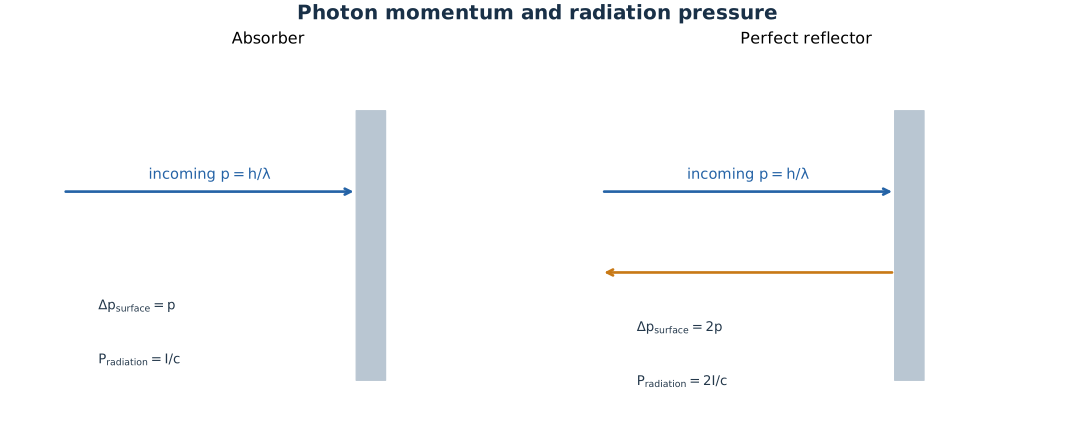
Absorption transfers one photon momentum; reversal by an ideal mirror transfers twice that momentum.

Problem 2.39 — derive the photon-energy wavelength shortcut

Paraphrased task. Derive the photon-energy wavelength shortcut.

Formula reference. Use (4), its definitions, and the topic illustration.

Worked application.

1. Start with \(E_\gamma=hc/\lambda\) in joules. To express the result in electron volts, divide by \(e=1.602176634\times10^{-19}\,\mathrm{J/eV}\).

2. If the numeric wavelength is in nanometres, its metre value is \(10^{-9}\lambda_{\rm nm}\).

3. Collect the constants:

   \[E_{\rm eV}=\frac{hc\,10^9/e}{\lambda_{\rm nm}} =\frac{1239.84}{\lambda_{\rm nm}}.\]

   The numerator has units eV nm, which cancel the denominator’s length unit.

Result. \(E_\gamma(\mathrm{eV})=1239.84/\lambda(\mathrm{nm})\).

Check. A 500 nm photon carries about 2.48 eV; using metres directly in this shortcut would be off by nine orders of magnitude.

Problem 2.40 — calculate solar radiation pressure for reflection

Paraphrased task. Calculate solar radiation pressure for reflection.

Formula reference. Use (4), its definitions, and the topic illustration.

Worked application.

1. Convert the incident solar flux with the conversion specified in the problem:

   \[I=\frac{2}{0.239}\frac{10^4}{60} =1.395\times10^3\,\mathrm{W/m^2}.\]

2. A photon reflected normally reverses its momentum, so the pressure is \(p=2I/c\).

3. Insert the flux: \(p=2(1395)/(3.00\times10^8)=9.30\times10^{-6}\,\mathrm{Pa}\), approximately \(9.2\times10^{-11}\) atmosphere. This follows the stated calories-to-joules conversion; 9.8 microPa is not obtained from these inputs.

Result. \(p\simeq9.3\times10^{-6}\,\mathrm{N/m^2}\) for perfect reflection.

Check. Replacing the mirror by a perfect absorber halves the pressure.

Problem 2.41 — find the photoelectric threshold wavelength

Paraphrased task. Find the photoelectric threshold wavelength.

Formula reference. Use (4), its definitions, and the topic illustration.

Worked application.

1. The threshold condition is \(E_\gamma=W\), with sodium work function \(W=1.8\,\mathrm{eV}\). Longer wavelengths have insufficient photon energy.

2. Solve \(hc/\lambda_{\max}=W\) for wavelength.

3. Using the photon-energy shortcut gives \(\lambda_{\max}=1239.84/1.8=688.8\,\mathrm{nm}\). Using the book’s rounded numerator 1239 gives 688.3 nm.

Result. The threshold wavelength is approximately \(689\,\mathrm{nm}\).

Check. Increasing intensity below the single-photon threshold does not change the energy of each photon in this model.

Problem 2.42 — find flashlight recoil thrust

Paraphrased task. Find flashlight recoil thrust.

Formula reference. Use (4), its definitions, and the topic illustration.

Worked application.

1. The flashlight emits energy \(P\Delta t\) in time \(\Delta t\), corresponding to forward photon momentum \(P\Delta t/c\).

2. Conservation of momentum gives equal and opposite flashlight recoil; divide by \(\Delta t\) to obtain \(F=P/c\).

3. With \(P=10^{-3}\,\mathrm W\), \(F=10^{-3}/(2.998\times10^8)=3.34\times10^{-12}\,\mathrm N\). There is no factor two because this is emission, not reversal of an incident beam.

Result. The recoil is \(3.34\times10^{-12}\,\mathrm N\) opposite the emitted beam.

Check. The force has dimensions \((\mathrm{J/s})/(\mathrm{m/s})=\mathrm N\); the scan’s printed larger value is inconsistent with 1 mW.

Problem 2.43 — find laser force on a reflecting microsphere

Paraphrased task. Find laser force on a reflecting microsphere.

Formula reference. Use (4), its definitions, and the topic illustration.

Worked application.

1. The reflecting surface area is \(9\times10^{-2}\,\mathrm{cm^2}=9\,\mathrm{mm^2}\), larger than the \(4\,\mathrm{mm^2}\) beam footprint. With full overlap it intercepts all 600 W.

2. The flux is \(I=600/(4\times10^{-6})=1.5\times10^8\,\mathrm{W/m^2}\). Perfect reflection gives \(p=2I/c\simeq1.00\,\mathrm{Pa}\).

3. Multiply by the illuminated beam area, not the entire larger reflector: \(F=p(4\times10^{-6})=4.00\times10^{-6}\,\mathrm N\).

Result. \(F=4.00\times10^{-6}\,\mathrm N\) along the incident beam.

Check. The same result follows directly from \(F=2P/c\).

Electromagnetic-photon spectrum

Formula and definitions.

(5)\[\nu=\frac{c}{\lambda},\qquad T=\frac{1}{\nu}=\frac{\lambda}{c},\qquad E_\gamma=\frac{hc}{\lambda},\qquad N=\frac{E_{\rm total}}{E_\gamma}\]

Classify the radiation from its wavelength or frequency, then use the vacuum dispersion relation. Photon count is total energy divided by the single-photon energy; convert \(1\,\mathrm{erg}=10^{-7}\,\mathrm J\) before division.

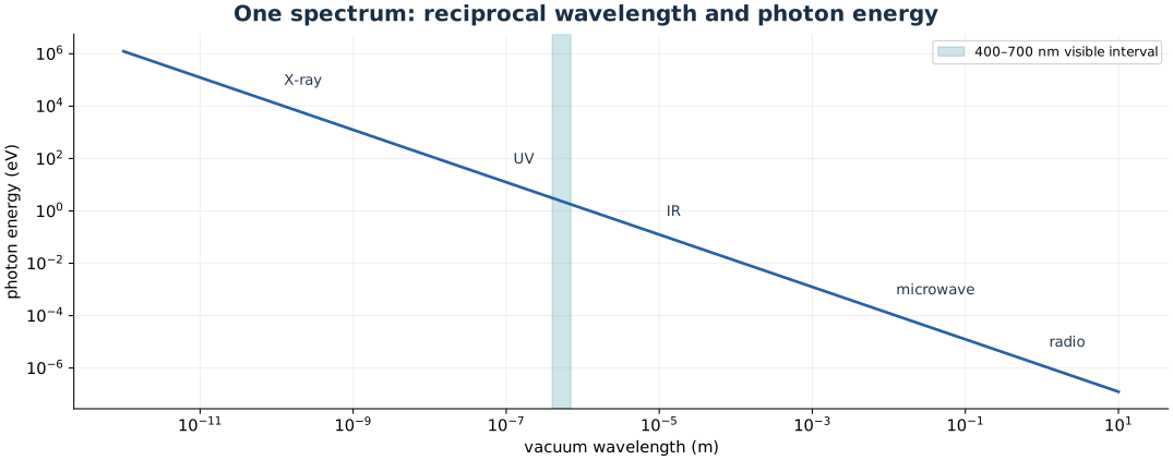
Photon energy decreases as wavelength increases. The visible band occupies only a small portion of this logarithmic scale.

Problem 2.44 — classify and quantify the 21-cm hydrogen line

Paraphrased task. Classify and quantify the 21-cm hydrogen line.

Formula reference. Use (5), its definitions, and the topic illustration.

Worked application.

1. Convert \(21\,\mathrm{cm}=0.21\,\mathrm m\).

2. The frequency is \(\nu=c/\lambda=2.998\times10^8/0.21=1.428\times10^9\,\mathrm{Hz}\).

3. Multiply by Planck’s constant: \(E_\gamma=h\nu=(6.626\times10^{-34})(1.428\times10^9)=9.46\times10^{-25}\,\mathrm J\). This is a microwave/radio spectral line, far below optical photon energies.

Result. \(\nu\simeq1.43\,\mathrm{GHz}\), \(E_\gamma\simeq9.46\times10^{-25}\,\mathrm J\).

Check. The energy is also \(5.90\times10^{-6}\,\mathrm{eV}\), consistent with a long wavelength.

Problem 2.45 — characterize extremely long radio waves

Paraphrased task. Characterize extremely long radio waves.

Formula reference. Use (5), its definitions, and the topic illustration.

Worked application.

1. Convert the given \(18{,}600{,}000\) miles using \(1609.344\,\mathrm{m/mile}\): \(\lambda=2.994\times10^{10}\,\mathrm m\).

2. The period is \(T=\lambda/c\simeq99.85\,\mathrm s\); the frequency is only about \(0.0100\,\mathrm{Hz}\).

3. Use \(E=h/T\) and divide by the joules-per-electron-volt conversion, obtaining \(E\simeq4.14\times10^{-17}\,\mathrm{eV}\).

Result. These extremely low-frequency radio waves have period about 100 s and photon energy \(4.14\times10^{-17}\,\mathrm{eV}\).

Check. An enormous wavelength implies both a long period and a very small photon energy.

Problem 2.46 — count photons carrying one erg at three wavelengths

Paraphrased task. Count photons carrying one erg at three wavelengths.

Formula reference. Use (5), its definitions, and the topic illustration.

Worked application.

1. One erg is \(U=10^{-7}\,\mathrm J\). The required photon count is \(N=U/E_\gamma=U\lambda/(hc)\).

2. Insert \(hc=1.98645\times10^{-25}\,\mathrm{J\,m}\) separately for the three wavelengths:

   \[N_\gamma=5.03\times10^5,\qquad N_{500\,\mathrm{nm}}=2.52\times10^{11},\qquad N_{1\,\mathrm{cm}}=5.03\times10^{15}.\]

3. The large change in count follows from keeping total energy fixed while increasing wavelength.

Result. Approximately \(5.0\times10^5\), \(2.5\times10^{11}\), and \(5.0\times10^{15}\) photons.

Check. Multiplying each count by \(hc/\lambda\) returns \(10^{-7}\,\mathrm J\).

Problem 2.47 — compare microwave and helium-neon photon energies

Paraphrased task. Compare microwave and helium-neon photon energies.

Formula reference. Use (5), its definitions, and the topic illustration.

Worked application.

1. Convert the two wavelengths to \(0.10\,\mathrm m\) and \(632.9\times10^{-9}\,\mathrm m\).

2. Divide \(hc=1.98645\times10^{-25}\,\mathrm{J\,m}\) by each wavelength to obtain \(1.986\times10^{-24}\,\mathrm J\) and \(3.139\times10^{-19}\,\mathrm J\).

3. Their ratio can be found without Planck’s constant: \(E_{\rm microwave}/E_{\rm HeNe}=\lambda_{\rm HeNe}/\lambda_{\rm microwave}=6.329\times10^{-6}\).

Result. The He–Ne photon carries approximately \(1.58\times10^5\) times the energy of the microwave photon.

Check. The shorter wavelength must correspond to the larger photon energy.