Chapter 8: Guided-Wave Optics

Source: Saleh and Teich, Fundamentals of Photonics, second edition, Chapter 8. These solutions retain the intermediate algebra so that every boundary condition, mode count, and numerical result can be checked.

Shared notation and conventions

The phasor convention is \(e^{j\omega t}\) with guided-wave factor \(e^{-j\beta z}\). The vacuum quantities are \(\lambda_0\) and \(k_0=2\pi/\lambda_0\); in a core of index \(n_1\), \(\lambda=\lambda_0/n_1\). The bounce angle \(\theta\) is measured from the guide axis, so

(1)\[\bar\theta_c=\cos^{-1}\!\left(\frac{n_2}{n_1}\right), \qquad \mathrm{NA}=n_1\sin\bar\theta_c =\sqrt{n_1^2-n_2^2}.\]

For a symmetric slab of full width \(d\), define

(2)\[k_y=n_1k_0\sin\theta,\quad \gamma=\sqrt{\beta^2-n_2^2k_0^2},\quad u=\frac{k_yd}{2},\quad w=\frac{\gamma d}{2},\quad V=\frac{k_0d}{2}\mathrm{NA},\qquad u^2+w^2=V^2.\]

Here scalar \(u\) is a dimensionless transverse phase, whereas \(u_m(y)\) is the book’s normalized mode function, \(\int|u_m(y)|^2dy=1\).

In-text exercises

Exercise 8.1-1 — Modal power

Brief solution

1. Method. We use vector-calculus identities, complex phasors, and integration identities.

2. Key step.

\[H_{y,m}=\frac{\beta_m}{\omega\mu} a_mu_m(y)e^{-j\beta_mz}.\]

\[\begin{split}\begin{aligned} P_{z,m} &=\frac12\operatorname{Re}\int E_{x,m}H_{y,m}^*dy\\ &=\frac12\frac{\beta_m}{\omega\mu}|a_m|^2 \int|u_m(y)|^2dy\\ &=\frac{|a_m|^2}{2}\frac{n/c_0}{\mu}\cos\theta_m. \end{aligned}\end{split}\]

Since \((n/c_0)/\mu=\sqrt{\epsilon/\mu}=1/\eta\),

3. Answer.

\[\boxed{P_{z,m}=\frac{|a_m|^2}{2\eta}\cos\theta_m}.\]

Show detailed stepsHide detailed steps

Step 1 — Definitions and setup. The TE modal field is

(3)\[\boldsymbol E_m=\hat{\boldsymbol x}\,a_mu_m(y)e^{-j\beta_mz}, \qquad \int|u_m(y)|^2dy=1,\]

where \(\beta_m=n(\omega/c_0)\cos\theta_m\) and \(\eta=\sqrt{\mu/\epsilon}=\eta_0/n\). Power is per unit length in the invariant \(x\) direction.

Figure 56 — Exercise 8.1-1: Modal power. The normalized transverse field and axial propagation constant determine the integrated Poynting flux.

Step 2 — Mathematical formulas used. We use vector-calculus identities, complex phasors, and integration identities.

Step 3 — Derive the associated magnetic field. From \(\nabla\times\boldsymbol E=-j\omega\mu\boldsymbol H\),

(4)\[H_{y,m}=\frac{\beta_m}{\omega\mu} a_mu_m(y)e^{-j\beta_mz}.\]

The sign gives positive axial flux because \(\hat{\boldsymbol x}\times\hat{\boldsymbol y} =\hat{\boldsymbol z}\).

Step 4 — Integrate the time-averaged Poynting vector.

(5)\[\begin{split}\begin{aligned} P_{z,m} &=\frac12\operatorname{Re}\int E_{x,m}H_{y,m}^*dy\\ &=\frac12\frac{\beta_m}{\omega\mu}|a_m|^2 \int|u_m(y)|^2dy\\ &=\frac{|a_m|^2}{2}\frac{n/c_0}{\mu}\cos\theta_m. \end{aligned}\end{split}\]

Since \((n/c_0)/\mu=\sqrt{\epsilon/\mu}=1/\eta\),

(6)\[\boxed{P_{z,m}=\frac{|a_m|^2}{2\eta}\cos\theta_m}.\]

Step 5 — Check. At \(\theta_m=0\) this is the plane-wave value; as \(\theta_m\to90^\circ\), the axial power tends to zero. The result has units \(|a_m|^2/\eta=\mathrm W\) under the modal normalization.

Exercise 8.1-2 — Multimode power

Brief solution

1. Method. We use integration identities and complex phasors.

2. Key step.

\[\begin{split}\begin{aligned} P_z&=\frac12\operatorname{Re}\int E_xH_y^*dy\\ &=\frac12\operatorname{Re}\sum_m\sum_n \frac{\beta_n}{\omega\mu}a_ma_n^* e^{-j(\beta_m-\beta_n)z}\int u_m(y)u_n(y)dy. \end{aligned}\end{split}\]

The Kronecker delta removes every \(m\ne n\) cross term, and the phase of each surviving diagonal term is unity:

\[P_z=\frac12\sum_m\frac{\beta_m}{\omega\mu}|a_m|^2.\]

3. Answer.

\[\boxed{P_z=\sum_m\frac{|a_m|^2}{2\eta}\cos\theta_m}.\]

Show detailed stepsHide detailed steps

Step 1 — Definitions and setup.

(7)\[E_x=\sum_m a_mu_m(y)e^{-j\beta_mz},\qquad H_y=\sum_n\frac{\beta_n}{\omega\mu} a_nu_n(y)e^{-j\beta_nz},\]

and the real mirror-guide modes obey \(\int u_m(y)u_n(y)dy=\delta_{mn}\).

Figure 57 — Exercise 8.1-2: Multimode power. Orthogonal modes add in field amplitude, while their integrated powers add without cross terms.

Step 2 — Mathematical formulas used. We use integration identities and complex phasors.

Step 3 — Expand before using orthogonality.

(8)\[\begin{split}\begin{aligned} P_z&=\frac12\operatorname{Re}\int E_xH_y^*dy\\ &=\frac12\operatorname{Re}\sum_m\sum_n \frac{\beta_n}{\omega\mu}a_ma_n^* e^{-j(\beta_m-\beta_n)z}\int u_m(y)u_n(y)dy. \end{aligned}\end{split}\]

The Kronecker delta removes every \(m\ne n\) cross term, and the phase of each surviving diagonal term is unity:

(9)\[P_z=\frac12\sum_m\frac{\beta_m}{\omega\mu}|a_m|^2.\]

Step 4 — Substitute the single-mode result.

(10)\[\boxed{P_z=\sum_m\frac{|a_m|^2}{2\eta}\cos\theta_m}.\]

Step 5 — Check. With only \(a_q\ne0\), this reduces to Exercise 8.1-1. It is independent of \(z\), as required in a lossless guide.

Exercise 8.2-1 — Slab confinement

Brief solution

1. Method. We use integration identities, trigonometric identities, and exponential identities.

2. Key step.

\[I_{\rm core}=\frac d2+\sigma_m\frac{\sin Q}{2k_y} =\frac d2\left(1+\sigma_m\frac{\sin Q}{Q}\right),\]

\[Q=2\pi\frac d\lambda\sin\theta_m,\qquad G=\gamma d=2\pi\frac d\lambda \sqrt{\sin^2\bar\theta_c-\sin^2\theta_m}.\]

Therefore

3. Answer.

\[\boxed{\Gamma_m=\left[ 1+\frac{1+\sigma_m\cos Q} {G(1+\sigma_m\sin Q/Q)}\right]^{-1}}, \qquad \sigma_m=(-1)^m.\]

Show detailed stepsHide detailed steps

Step 1 — Definitions and setup. Use the unnormalized symmetric-slab profile

(11)\[\begin{split}f_m(y)= \begin{cases} \cos(k_yy),&|y|\le d/2,\ m\ \text{even},\\ \sin(k_yy),&|y|\le d/2,\ m\ \text{odd},\\ f_m(d/2)e^{-\gamma(y-d/2)},&y>d/2, \end{cases}\end{split}\]

with even or odd continuation below. Normalization cancels from \(\Gamma_m=P_{\rm core}/P_{\rm total}\).

Figure 58 — Exercise 8.2-1: Slab confinement. The harmonic core power is compared with both evanescent tails.

Step 2 — Mathematical formulas used. We use integration identities, trigonometric identities, and exponential identities.

Step 3 — Integrate the core. Let \(\sigma_m=(-1)^m\) and \(Q=k_yd\). The even and odd cases combine as

(12)\[I_{\rm core}=\frac d2+\sigma_m\frac{\sin Q}{2k_y} =\frac d2\left(1+\sigma_m\frac{\sin Q}{Q}\right),\]

while the boundary intensity is

(13)\[|f_m(d/2)|^2=\frac{1+\sigma_m\cos Q}{2}.\]

Step 4 — Integrate both tails.

(14)\[I_{\rm clad}=2|f_m(d/2)|^2\int_0^\infty e^{-2\gamma s}ds =\frac{|f_m(d/2)|^2}{\gamma}.\]

Express the transverse phase and decay only through the requested variables:

(15)\[Q=2\pi\frac d\lambda\sin\theta_m,\qquad G=\gamma d=2\pi\frac d\lambda \sqrt{\sin^2\bar\theta_c-\sin^2\theta_m}.\]

Therefore

(16)\[\boxed{\Gamma_m=\left[ 1+\frac{1+\sigma_m\cos Q} {G(1+\sigma_m\sin Q/Q)}\right]^{-1}}, \qquad \sigma_m=(-1)^m.\]

Step 5 — Check. Increasing \(m\) increases \(\theta_m\), decreases \(\gamma\), and increases the tail length \(1/\gamma\), which diverges at cutoff. Thus the nodeless \(m=0\) mode has the greatest confinement. The limit \(\gamma\to0^+\) correctly gives \(\Gamma_m\to0\) near cutoff.

Exercise 8.2-2 — Asymmetric slab

Brief solution

1. Method. We use trigonometric identities and algebraic rearrangement.

2. Key step.

\[\tan\frac{\phi_{1j}}2 =\sqrt{\frac{\sin^2\bar\theta_{cj}}{\sin^2\theta}-1}, \qquad j=2,3.\]

One round trip contains one reflection at each boundary, so

3. Answer.

\[\boxed{\theta_{\max}=\cos^{-1}(n_2/n_1)}, \qquad \boxed{\mathrm{NA}=n_1\sin\theta_{\max} =\sqrt{n_1^2-n_2^2}}.\]

\[\boxed{2k_yd-\phi_{12}-\phi_{13}=2\pi m}, \qquad k_y=\frac{2\pi}{\lambda}\sin\theta.\]

When \(n_3=n_2\), the two phases become equal and the symmetric-slab condition is recovered.

Show detailed stepsHide detailed steps

Step 1 — Definitions and setup. The core, substrate, and cover indices are \(n_1\), \(n_2\), and \(n_3\), with \(n_3<n_2<n_1\).

Figure 59 — Exercise 8.2-2: Asymmetric slab. The higher-index substrate sets the stricter ray limit; the two boundaries contribute unequal reflection phases.

Step 2 — Mathematical formulas used. We use trigonometric identities and algebraic rearrangement.

Step 3 — Part (a): maximum angle and NA. Since \(\cos\bar\theta_{cj}=n_j/n_1\) and \(n_2>n_3\), the substrate has the smaller complementary critical angle:

(17)\[\boxed{\theta_{\max}=\cos^{-1}(n_2/n_1)}, \qquad \boxed{\mathrm{NA}=n_1\sin\theta_{\max} =\sqrt{n_1^2-n_2^2}}.\]

Step 4 — Part (b): self-consistency. For TE polarization define

(18)\[\tan\frac{\phi_{1j}}2 =\sqrt{\frac{\sin^2\bar\theta_{cj}}{\sin^2\theta}-1}, \qquad j=2,3.\]

One round trip contains one reflection at each boundary, so

(19)\[\boxed{2k_yd-\phi_{12}-\phi_{13}=2\pi m}, \qquad k_y=\frac{2\pi}{\lambda}\sin\theta.\]

When \(n_3=n_2\), the two phases become equal and the symmetric-slab condition is recovered.

Step 5 — Part (c): many-mode limit. Reflection phase changes shift the endpoints only by order unity. With approximate spacing \(\Delta(\sin\theta)=\lambda/(2d)\),

(20)\[\boxed{M\simeq\frac{2d}{\lambda}\sin\theta_{\max} =\frac{2d}{\lambda_0}\sqrt{n_1^2-n_2^2}},\qquad M\gg1.\]

The cover still changes individual propagation constants, but the higher-index substrate controls the leading mode count.

Check. Setting \(n_3=n_2\) recovers both the symmetric phase condition and its symmetric large-mode count.

End-of-chapter problems

Problem 8.1-3 — Mirror-guide field

Brief solution

1. Method. We use complex-exponential identities and algebraic rearrangement.

2. Key step.

\[E_x(d/2,z)=Ae^{-jk_yd/2}e^{-j\beta z}=0.\]

\[A_1e^{-jqd/2}+A_2e^{jqd/2}=0,\qquad A_1e^{jqd/2}+A_2e^{-jqd/2}=0.\]

The first boundary equation then fixes the relative sign:

3. Answer.

\[e^{-jqd}-e^{jqd}=-2j\sin(qd)=0 \quad\Longrightarrow\quad \boxed{q=k_y=\frac{m\pi}{d}},\quad m=1,2,\ldots.\]

\[\boxed{\frac{A_2}{A_1}=-e^{-jqd}=(-1)^{m+1}}.\]

Odd \(m\) therefore gives \(A_2=A_1\) and a cosine mode; even \(m\) gives \(A_2=-A_1\) and a sine mode.

Show detailed stepsHide detailed steps

Definitions and setup. The perfect mirrors are at \(y=\pm d/2\); both boundary values must vanish for every \(z\).

Mathematical formulas used. We use complex-exponential identities and algebraic rearrangement.

Worked derivation.

Part (a): test one plane wave. At the upper mirror,

(21)\[E_x(d/2,z)=Ae^{-jk_yd/2}e^{-j\beta z}=0.\]

The exponentials never vanish, so \(A=0\). A nonzero single traveling wave cannot form nodes at both mirrors.

Part (b): impose both boundaries on two waves. Set \(k_{y1}=q\), \(k_{y2}=-q\), and \(\beta_1=\beta_2=\beta\). Using complex-exponential identities,

(22)\[E_x=e^{-j\beta z}\left(A_1e^{-jqy}+A_2e^{jqy}\right).\]

The equations at \(y=+d/2\) and \(y=-d/2\) are

(23)\[A_1e^{-jqd/2}+A_2e^{jqd/2}=0,\qquad A_1e^{jqd/2}+A_2e^{-jqd/2}=0.\]

A nonzero solution requires the determinant to vanish:

(24)\[e^{-jqd}-e^{jqd}=-2j\sin(qd)=0 \quad\Longrightarrow\quad \boxed{q=k_y=\frac{m\pi}{d}},\quad m=1,2,\ldots.\]

The first boundary equation then fixes the relative sign:

(25)\[\boxed{\frac{A_2}{A_1}=-e^{-jqd}=(-1)^{m+1}}.\]

Odd \(m\) therefore gives \(A_2=A_1\) and a cosine mode; even \(m\) gives \(A_2=-A_1\) and a sine mode.

Note

The printed problem says the sum “does not satisfy” the boundaries under these conditions. Direct substitution shows that an arbitrary \(\pm\) sign fails, but the parity-matched sign above satisfies both mirrors. This appears to be a wording error in the printed question.

Check. \(\cos(m\pi y/d)\) vanishes at both mirrors for odd \(m\), while \(\sin(m\pi y/d)\) vanishes there for even \(m\).

Problem 8.1-4 — Mirror-guide dispersion

Brief solution

1. Method. We use the chain rule and algebraic and dimensional checks.

2. Key step.

There are 62 polarization-resolved modes. The book’s mirror-guide sequence starts at \(m=1\), not at a TEM \(m=0\) endpoint.

\[v_{g,m}=\left(\frac{d\beta_m}{d\omega}\right)^{-1} =\frac{c_0}{n}\sqrt{1-\left(\frac{m\lambda}{2d}\right)^2}.\]

The fastest and slowest modes are \(m=1\) and \(m=31\):

3. Answer.

\[\frac{2d}{\lambda}=\frac{20}{0.633}=31.5956 \quad\Longrightarrow\quad \boxed{M_{\rm TE}=31,\qquad M_{\rm TM}=31}.\]

\[\begin{split}\begin{aligned} v_{g,1}&=c_0\sqrt{1-(0.633/20)^2} =\boxed{2.99642\times10^8\ \mathrm{m\,s^{-1}}},\\ v_{g,31}&=c_0\sqrt{1-(31\times0.633/20)^2} =\boxed{5.79342\times10^7\ \mathrm{m\,s^{-1}}}. \end{aligned}\end{split}\]

\[\begin{split}\begin{aligned} \Delta t &=L\left(\frac1{v_{g,31}}-\frac1{v_{g,1}}\right)\\ &=1.726096\times10^{-8}-3.337313\times10^{-9}\ \mathrm s\\ &=\boxed{13.924\ \mathrm{ns}}. \end{aligned}\end{split}\]

The high-order zigzag ray follows the longer path, so the positive delay is also the expected physical sign.

Show detailed stepsHide detailed steps

Definitions and setup. \(\lambda_0=0.633\ \mu\mathrm m\), \(d=10\ \mu\mathrm m\), and \(n=1\), hence \(\lambda=\lambda_0/n=0.633\ \mu\mathrm m\).

Mathematical formulas used. We use the chain rule and algebraic and dimensional checks.

Worked derivation.

Mode count. The guide permits \(m=1,\ldots,M\) with \(m\lambda/(2d)<1\). Thus

(26)\[\frac{2d}{\lambda}=\frac{20}{0.633}=31.5956 \quad\Longrightarrow\quad \boxed{M_{\rm TE}=31,\qquad M_{\rm TM}=31}.\]

There are 62 polarization-resolved modes. The book’s mirror-guide sequence starts at \(m=1\), not at a TEM \(m=0\) endpoint.

Derive the group velocity. With nondispersive \(n\),

(27)\[\beta_m^2=\left(\frac{n\omega}{c_0}\right)^2 -\left(\frac{m\pi}{d}\right)^2.\]

Differentiate using the chain rule:

(28)\[v_{g,m}=\left(\frac{d\beta_m}{d\omega}\right)^{-1} =\frac{c_0}{n}\sqrt{1-\left(\frac{m\lambda}{2d}\right)^2}.\]

The fastest and slowest modes are \(m=1\) and \(m=31\):

(29)\[\begin{split}\begin{aligned} v_{g,1}&=c_0\sqrt{1-(0.633/20)^2} =\boxed{2.99642\times10^8\ \mathrm{m\,s^{-1}}},\\ v_{g,31}&=c_0\sqrt{1-(31\times0.633/20)^2} =\boxed{5.79342\times10^7\ \mathrm{m\,s^{-1}}}. \end{aligned}\end{split}\]

Pulse spread over 1 m.

(30)\[\begin{split}\begin{aligned} \Delta t &=L\left(\frac1{v_{g,31}}-\frac1{v_{g,1}}\right)\\ &=1.726096\times10^{-8}-3.337313\times10^{-9}\ \mathrm s\\ &=\boxed{13.924\ \mathrm{ns}}. \end{aligned}\end{split}\]

The high-order zigzag ray follows the longer path, so the positive delay is also the expected physical sign.

Check. Both velocities lie between zero and \(c_0\), and direct substitution of them in \(L/v_g\) reproduces the stated delay.

Problem 8.2-3 — Film in index-1.4 cladding

Brief solution

1. Method. We use trigonometric identities, the chain rule, and algebraic rearrangement.

2. Key step.

At an air entrance face, Snell’s law gives \(\sin\theta_{a,\max}=\mathrm{NA}\), hence

\[\frac{d\beta}{dk_0}= \frac{n_1^2k_0-(2u\,\mathrm{NA}/d)(du/dV)}{\beta}.\]

Since \(\omega=c_0k_0\),

3. Answer.

\[\begin{split}\begin{aligned} \theta_c&=\sin^{-1}(1.4/1.6)=\boxed{61.045^\circ},\\ \bar\theta_c&=90^\circ-\theta_c=\boxed{28.955^\circ},\\ \mathrm{NA}&=\sqrt{1.6^2-1.4^2}=\boxed{0.774597}. \end{aligned}\end{split}\]

\[\boxed{\theta_{a,\max}=\sin^{-1}(0.774597)=50.768^\circ}.\]

\[\frac{2d\,\mathrm{NA}}{\lambda_0}=3.56136 \quad\Longrightarrow\quad \boxed{M_{\rm TE}=4}.\]

\[\boxed{\theta_0=\sin^{-1}\!\left( \frac{u\lambda_0}{\pi n_1d}\right)=6.61249^\circ}.\]

\[\boxed{v_g=\frac{c_0}{d\beta/dk_0} =1.86508\times10^8\ \mathrm{m\,s^{-1}}}.\]

The simpler ray estimate \((c_0/n_1)\cos\theta_0 =1.86124\times10^8\ \mathrm{m/s}\) differs by 0.21%; the exact derivative includes the frequency-dependent reflection-phase delay.

Show detailed stepsHide detailed steps

Definitions and setup. \(\lambda_0=0.87\ \mu\mathrm m\), \(d=2.00\ \mu\mathrm m\), \(n_1=1.60\), and \(n_2=1.40\).

Mathematical formulas used. We use trigonometric identities, the chain rule, and algebraic rearrangement.

Worked derivation.

Part (a): angles and aperture.

(31)\[\begin{split}\begin{aligned} \theta_c&=\sin^{-1}(1.4/1.6)=\boxed{61.045^\circ},\\ \bar\theta_c&=90^\circ-\theta_c=\boxed{28.955^\circ},\\ \mathrm{NA}&=\sqrt{1.6^2-1.4^2}=\boxed{0.774597}. \end{aligned}\end{split}\]

At an air entrance face, Snell’s law gives \(\sin\theta_{a,\max}=\mathrm{NA}\), hence

(32)\[\boxed{\theta_{a,\max}=\sin^{-1}(0.774597)=50.768^\circ}.\]

Part (b): TE mode count. The chapter uses the smallest integer greater than \(2d\,\mathrm{NA}/\lambda_0\):

(33)\[\frac{2d\,\mathrm{NA}}{\lambda_0}=3.56136 \quad\Longrightarrow\quad \boxed{M_{\rm TE}=4}.\]

Part (c): TE0 eigenvalue and angle.

(34)\[V=\frac{\pi d}{\lambda_0}\mathrm{NA}=5.594177,\qquad u\tan u=\sqrt{V^2-u^2}.\]

Solving on \(0<u<\pi/2\) gives \(u=1.3306338\), \(w=5.4336208\), and

(35)\[\boxed{\theta_0=\sin^{-1}\!\left( \frac{u\lambda_0}{\pi n_1d}\right)=6.61249^\circ}.\]

Group velocity including waveguide dispersion. Let \(F(u,V)=u\tan u-\sqrt{V^2-u^2}=0\). Implicit differentiation gives

(36)\[\frac{du}{dV}= \frac{V/w}{\tan u+u\sec^2u+u/w}=0.0369715.\]

Using \(\beta=[n_1^2k_0^2-(2u/d)^2]^{1/2}\) and \(du/dk_0=(d\,\mathrm{NA}/2)(du/dV)\), the chain rule gives

(37)\[\frac{d\beta}{dk_0}= \frac{n_1^2k_0-(2u\,\mathrm{NA}/d)(du/dV)}{\beta}.\]

Since \(\omega=c_0k_0\),

(38)\[\boxed{v_g=\frac{c_0}{d\beta/dk_0} =1.86508\times10^8\ \mathrm{m\,s^{-1}}}.\]

The simpler ray estimate \((c_0/n_1)\cos\theta_0 =1.86124\times10^8\ \mathrm{m/s}\) differs by 0.21%; the exact derivative includes the frequency-dependent reflection-phase delay.

Check. The root obeys \(u\tan u=w\) to the shown precision and \(\theta_0<\bar\theta_c\). The exact group velocity is close to the ray estimate and may lie slightly below \(c_0/n_1\), as expected from the chapter’s waveguide-dispersion curve.

Problem 8.2-4 — Film suspended in air

Brief solution

1. Method. We use trigonometric identities, the implicit chain rule, and algebraic rearrangement.

2. Key step.

Repeating (36)– (37) with \(du/dV=0.0158137\) yields

3. Answer.

\[\theta_c=\boxed{38.682^\circ},\qquad \bar\theta_c=\boxed{51.318^\circ},\qquad \mathrm{NA}=\boxed{1.24900}.\]

The formal entrance relation \(\sin\theta_a=1.249>1\) means the guide accepts the entire propagating angular range available in air: \(\boxed{\theta_{a,\max}=90^\circ}\) in the ideal end-face model.

\[\frac{2d\,\mathrm{NA}}{\lambda_0}=5.74253 \quad\Longrightarrow\quad \boxed{M_{\rm TE}=6}.\]

\[V=9.020340,\qquad u=1.4134518,\qquad w=8.9089107,\qquad \boxed{\theta_0=7.02606^\circ}.\]

\[\boxed{v_g=1.86244\times10^8\ \mathrm{m\,s^{-1}}}.\]

The ray estimate is \(1.85963\times10^8\ \mathrm{m/s}\). Relative to Problem 8.2-3, air cladding increases the mode count from 4 to 6 and raises the TE0 confinement from 99.12% to 99.75%, while changing its angle and group velocity only slightly.

Show detailed stepsHide detailed steps

Definitions and setup. Keep the preceding \(\lambda_0,d,n_1\), but set \(n_2=1\).

Mathematical formulas used. We use trigonometric identities, the implicit chain rule, and algebraic rearrangement.

Worked derivation.

Part (a).

(39)\[\theta_c=\boxed{38.682^\circ},\qquad \bar\theta_c=\boxed{51.318^\circ},\qquad \mathrm{NA}=\boxed{1.24900}.\]

The formal entrance relation \(\sin\theta_a=1.249>1\) means the guide accepts the entire propagating angular range available in air: \(\boxed{\theta_{a,\max}=90^\circ}\) in the ideal end-face model.

Part (b).

(40)\[\frac{2d\,\mathrm{NA}}{\lambda_0}=5.74253 \quad\Longrightarrow\quad \boxed{M_{\rm TE}=6}.\]

Part (c). The even-mode equation gives

(41)\[V=9.020340,\qquad u=1.4134518,\qquad w=8.9089107,\qquad \boxed{\theta_0=7.02606^\circ}.\]

Repeating (36)– (37) with \(du/dV=0.0158137\) yields

(42)\[\boxed{v_g=1.86244\times10^8\ \mathrm{m\,s^{-1}}}.\]

The ray estimate is \(1.85963\times10^8\ \mathrm{m/s}\). Relative to Problem 8.2-3, air cladding increases the mode count from 4 to 6 and raises the TE0 confinement from 99.12% to 99.75%, while changing its angle and group velocity only slightly.

Check. The lower cladding index increases NA and therefore cannot decrease the mode count; all calculated angles remain within the TIR limit.

Problem 8.2-5 — TE0 field and confinement

Brief solution

1. Method. We use integration identities, exponential identities, and trigonometric identities.

2. Key step.

For even TE0, \(\varphi=0\), so \(B/A=e^w\cos u\).

\[\begin{split}u_0(y)=N\begin{cases} \cos(k_yy),&|y|\le d/2,\\ \cos u\,e^{-\gamma(|y|-d/2)},&|y|>d/2. \end{cases}\end{split}\]

\[\begin{split}\begin{aligned} N^{-2}&=\left[\frac d2+\frac{\sin(2u)}{2k_y}\right] +\frac{\cos^2u}{\gamma}\\ &=0.4728045+1.1741324=1.6469369\ \mu\mathrm m, \end{aligned}\end{split}\]

3. Answer.

\[A\cos(k_yd/2+\varphi)=Be^{-\gamma d/2} \quad\Longrightarrow\quad \boxed{\frac BA=e^{\gamma d/2}\cos(k_yd/2+\varphi)}.\]

so \(\boxed{N=0.779223\ \mu\mathrm m^{-1/2}}\).

\[\boxed{\Gamma_0=\frac{0.4728045}{0.4728045+1.1741324} =0.287081=28.71\%}.\]

This is plausible because \(V=0.448\ll1\) and the intensity decay length \(1/(2\gamma)=0.6985\ \mu\mathrm m\) exceeds the core half-width.

Show detailed stepsHide detailed steps

Definitions and setup. \(n_1=1.48\), \(n_2=1.46\), \(d=0.500\ \mu\mathrm m\), and \(\lambda_0=0.850\ \mu\mathrm m\).

Mathematical formulas used. We use integration identities, exponential identities, and trigonometric identities.

Worked derivation.

Ratio of proportionality constants. Matching the book’s \(A\cos(k_yy+\varphi)\) core field to \(Be^{-\gamma y}\) at \(y=d/2\) gives

(43)\[A\cos(k_yd/2+\varphi)=Be^{-\gamma d/2} \quad\Longrightarrow\quad \boxed{\frac BA=e^{\gamma d/2}\cos(k_yd/2+\varphi)}.\]

For even TE0, \(\varphi=0\), so \(B/A=e^w\cos u\).

Solve the eigenvalue.

(44)\[\mathrm{NA}=0.242487,\quad V=0.448115,\quad u\tan u=\sqrt{V^2-u^2} \Longrightarrow u=0.4108277,\ w=0.1789630.\]

Thus \(k_y=1.643311\ \mu\mathrm m^{-1}\), \(\gamma=0.715852\ \mu\mathrm m^{-1}\), and \(B/A=1.096460\). A continuous normalized profile is

(45)\[\begin{split}u_0(y)=N\begin{cases} \cos(k_yy),&|y|\le d/2,\\ \cos u\,e^{-\gamma(|y|-d/2)},&|y|>d/2. \end{cases}\end{split}\]

Using integration identities,

(46)\[\begin{split}\begin{aligned} N^{-2}&=\left[\frac d2+\frac{\sin(2u)}{2k_y}\right] +\frac{\cos^2u}{\gamma}\\ &=0.4728045+1.1741324=1.6469369\ \mu\mathrm m, \end{aligned}\end{split}\]

so \(\boxed{N=0.779223\ \mu\mathrm m^{-1/2}}\).

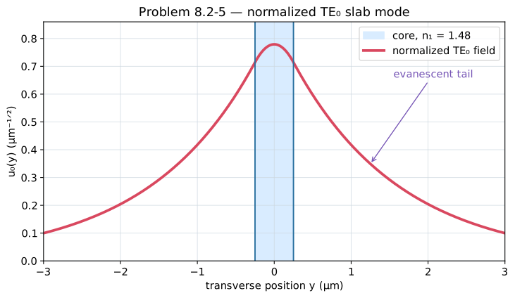
Figure 60 — Problem 8.2-5: normalized TE0 field. The shaded core is \(-0.25\le y\le0.25\ \mu\mathrm m\); field and slope are continuous at both interfaces.

Confinement. The factor \(N^2\) cancels, so

(47)\[\boxed{\Gamma_0=\frac{0.4728045}{0.4728045+1.1741324} =0.287081=28.71\%}.\]

This is plausible because \(V=0.448\ll1\) and the intensity decay length \(1/(2\gamma)=0.6985\ \mu\mathrm m\) exceeds the core half-width.

Check. Substitution of \(N\) makes the total field integral unity, and the core and cladding fractions sum to one.

Problem 8.2-6 — Maxwell derivation

Brief solution

1. Method. The curl, Helmholtz equation, exponential derivative, and electromagnetic boundary conditions are used below.

2. Key step.

Let \(\boldsymbol E=\hat{\boldsymbol x}u(y)e^{-j\beta z}\). With the \(e^{j\omega t}\) convention and vector-calculus identities,

\[\tan\left(\frac{k_yd}{2}-\frac{m\pi}{2}\right)=\frac{\gamma}{k_y}, \qquad \frac{\gamma}{k_y}=\sqrt{ \frac{\sin^2\bar\theta_c}{\sin^2\theta}-1}.\]

Because \(k_yd/2=\pi(d/\lambda)\sin\theta\), this becomes

3. Answer.

\[\boxed{H_y=\frac{\beta}{\omega\mu}u(y)e^{-j\beta z}}, \qquad \boxed{H_z=-\frac{j}{\omega\mu}u'(y)e^{-j\beta z}}.\]

\[\boxed{k_y\tan(k_yd/2)=\gamma} \quad\Longleftrightarrow\quad \boxed{u\tan u=w}.\]

\[\boxed{-k_y\cot(k_yd/2)=\gamma} \quad\Longleftrightarrow\quad \boxed{-u\cot u=w}.\]

\[\boxed{\tan\left(\pi\frac d\lambda\sin\theta_m-\frac{m\pi}{2}\right) =\sqrt{\frac{\sin^2\bar\theta_c}{\sin^2\theta_m}-1}},\]

which is Eq. (8.2-4). Derivative continuity is the step that turns a merely continuous trial field into a permitted eigenmode.

Show detailed stepsHide detailed steps

Definitions and setup. The TE field has one electric-field component; the media are nonmagnetic and the interfaces are parallel to the guide axis.

Mathematical formulas used. The curl, Helmholtz equation, exponential derivative, and electromagnetic boundary conditions are used below.

Worked derivation.

Let \(\boldsymbol E=\hat{\boldsymbol x}u(y)e^{-j\beta z}\). With the \(e^{j\omega t}\) convention and vector-calculus identities,

(48)\[\nabla\times\boldsymbol E =(0,-j\beta u,-u')e^{-j\beta z} =-j\omega\mu\boldsymbol H.\]

Therefore

(49)\[\boxed{H_y=\frac{\beta}{\omega\mu}u(y)e^{-j\beta z}}, \qquad \boxed{H_z=-\frac{j}{\omega\mu}u'(y)e^{-j\beta z}}.\]

The constant-coefficient ODE solutions applied to the Helmholtz equation require

(50)\[k_y^2+\beta^2=n_1^2k_0^2,\qquad -\gamma^2+\beta^2=n_2^2k_0^2.\]

Subtracting them and multiplying by \(d^2/4\) verifies \(u^2+w^2=V^2\).

Apply both boundary conditions. Equal permeabilities make continuity of tangential \(E_x,H_z\) equivalent to continuity of \(u,u'\). For an even core field at \(y=d/2\),

(51)\[A\cos(k_yd/2)=Be^{-\gamma d/2},\qquad -Ak_y\sin(k_yd/2)=-\gamma Be^{-\gamma d/2}.\]

Dividing the equations gives

(52)\[\boxed{k_y\tan(k_yd/2)=\gamma} \quad\Longleftrightarrow\quad \boxed{u\tan u=w}.\]

For odd \(A\sin(k_yy)\), the same operation yields

(53)\[\boxed{-k_y\cot(k_yd/2)=\gamma} \quad\Longleftrightarrow\quad \boxed{-u\cot u=w}.\]

Combine the parity cases and substitute the angle definitions:

(54)\[\tan\left(\frac{k_yd}{2}-\frac{m\pi}{2}\right)=\frac{\gamma}{k_y}, \qquad \frac{\gamma}{k_y}=\sqrt{ \frac{\sin^2\bar\theta_c}{\sin^2\theta}-1}.\]

Because \(k_yd/2=\pi(d/\lambda)\sin\theta\), this becomes

(55)\[\boxed{\tan\left(\pi\frac d\lambda\sin\theta_m-\frac{m\pi}{2}\right) =\sqrt{\frac{\sin^2\bar\theta_c}{\sin^2\theta_m}-1}},\]

which is Eq. (8.2-4). Derivative continuity is the step that turns a merely continuous trial field into a permitted eigenmode.

Check. Either parity profile recovers the two regional dispersion relations, and both tangential field components are continuous.

Problem 8.2-7 — Single-mode thickness

Brief solution

1. Method. The mode-count inequality and algebraic rearrangement are used below.

2. Key step.

For \(n_1=1.50\) and \(n_2=1.46\),

\[\mathrm{NA}=\sqrt{1.50^2-1.46^2}=0.344093.\]

At \(\lambda_0'=0.85\ \mu\mathrm m\), keeping this thickness,

3. Answer.

\[\boxed{d_{\max}=\frac{1.30}{2(0.344093)} =1.88902\ \mu\mathrm m}.\]

\[\frac{2d_{\max}\mathrm{NA}}{\lambda_0'} =\frac{1.30}{0.85}=1.52941 \quad\Longrightarrow\quad \boxed{M_{\rm TE}=2}.\]

The inverse-wavelength scaling confirms that the shorter wavelength must support more modes.

Show detailed stepsHide detailed steps

Definitions and setup. The guide is symmetric and material dispersion is not included.

Mathematical formulas used. The mode-count inequality and algebraic rearrangement are used below.

Worked derivation.

For \(n_1=1.50\) and \(n_2=1.46\),

(56)\[\mathrm{NA}=\sqrt{1.50^2-1.46^2}=0.344093.\]

The \(m=1\) branch reaches cutoff at \(2d\,\mathrm{NA}/\lambda_0=1\). At equality it is marginal and not evanescent outside, so the largest thickness retaining only confined TE0 is

(57)\[\boxed{d_{\max}=\frac{1.30}{2(0.344093)} =1.88902\ \mu\mathrm m}.\]

At \(\lambda_0'=0.85\ \mu\mathrm m\), keeping this thickness,

(58)\[\frac{2d_{\max}\mathrm{NA}}{\lambda_0'} =\frac{1.30}{0.85}=1.52941 \quad\Longrightarrow\quad \boxed{M_{\rm TE}=2}.\]

The inverse-wavelength scaling confirms that the shorter wavelength must support more modes.

Check. Substitution of the limiting thickness returns the first higher-order-mode cutoff, with dimensions of length.

Problem 8.2-8 — Cutoff approximation

Brief solution

1. Method. The cutoff phase condition, difference of squares, and weak-guidance approximation are used below.

2. Key step.

Let \(\Delta n=n_1-n_2\) and \(m>0\). At cutoff, \(\gamma\to0\), the reflection phase tends to zero, and \(\theta_m\to\bar\theta_c\). The phase condition reduces to

\[\lambda_{0,c}^2 =\frac{4d^2}{m^2}(n_1-n_2)(n_1+n_2).\]

For weak guidance \(n_2\simeq n_1\), hence \(n_1+n_2\simeq2n_1\) and

3. Answer.

\[\boxed{\lambda_{0,c}^2\simeq \frac{8n_1\Delta n\,d^2}{m^2}}.\]

Dimensions are length squared on both sides. Increasing \(d\) or index contrast correctly moves cutoff to a longer wavelength.

Show detailed stepsHide detailed steps

Definitions and setup. The index difference is small and the mode is a higher-order TE mode.

Mathematical formulas used. The cutoff phase condition, difference of squares, and weak-guidance approximation are used below.

Worked derivation.

Let \(\Delta n=n_1-n_2\) and \(m>0\). At cutoff, \(\gamma\to0\), the reflection phase tends to zero, and \(\theta_m\to\bar\theta_c\). The phase condition reduces to

(59)\[\frac{2\pi}{\lambda}(2d\sin\bar\theta_c)=2\pi m \quad\Longrightarrow\quad \frac{2d}{\lambda_0}\sqrt{n_1^2-n_2^2}=m.\]

Solving and factoring the difference of squares gives

(60)\[\lambda_{0,c}^2 =\frac{4d^2}{m^2}(n_1-n_2)(n_1+n_2).\]

For weak guidance \(n_2\simeq n_1\), hence \(n_1+n_2\simeq2n_1\) and

(61)\[\boxed{\lambda_{0,c}^2\simeq \frac{8n_1\Delta n\,d^2}{m^2}}.\]

Dimensions are length squared on both sides. Increasing \(d\) or index contrast correctly moves cutoff to a longer wavelength.

Check. Replacing the index sum by twice the core index in the exact result reproduces the approximation without changing dimensions.

Problem 8.2-9 — TM modes

Brief solution

1. Method. The TM total-internal-reflection phase, trigonometric identities, and algebraic rearrangement are used below.

2. Key step.

For total internal reflection of a TM wave,

\[\tan(5\pi s-m\pi/2)=1.098901\sqrt{0.09/s^2-1}.\]

The book’s count is the smallest integer strictly greater than \(s_c/[\lambda/(2d)]=3\), so

3. Answer.

\[\boxed{\tan\left(\pi\frac d\lambda\sin\theta_m-\frac{m\pi}{2}\right) =\frac{n_1^2}{n_2^2} \sqrt{\frac{\sin^2\bar\theta_c}{\sin^2\theta_m}-1}}.\]

\[\boxed{M_{\rm TM}=4}.\]

Only the first three have \(\gamma>0\); \(m=3\) is marginal at the specified exact cutoff. A plot that omits its endpoint will appear to show only three intersections.

Show detailed stepsHide detailed steps

Definitions and setup. The bounce angle is measured from the guide axis; the requested plot uses the sine of that angle.

Mathematical formulas used. The TM total-internal-reflection phase, trigonometric identities, and algebraic rearrangement are used below.

Worked derivation.

For total internal reflection of a TM wave,

(62)\[\tan\frac{\phi_{\rm TM}}2 =\frac{n_1^2}{n_2^2} \sqrt{\frac{\sin^2\bar\theta_c}{\sin^2\theta}-1}.\]

Substitute this in \(2k_yd-2\phi_{\rm TM}=2\pi m\) and take the tangent of the half-phase equation:

(63)\[\boxed{\tan\left(\pi\frac d\lambda\sin\theta_m-\frac{m\pi}{2}\right) =\frac{n_1^2}{n_2^2} \sqrt{\frac{\sin^2\bar\theta_c}{\sin^2\theta_m}-1}}.\]

The index-squared factor is the difference from TE polarization. For \(s=\sin\theta\), \(s_c=0.3\), and \(\lambda/(2d)=0.1\), one has \(d/\lambda=5\) and \(n_1^2/n_2^2=1/(1-s_c^2)=1.098901\). The numerical equation is

(64)\[\tan(5\pi s-m\pi/2)=1.098901\sqrt{0.09/s^2-1}.\]

TM branch intersections

\(m\)	\(\sin\theta_m\)	\(\theta_m\)	status
0	0.0835713	\(4.79387^\circ\)	guided
1	0.165506	\(9.52662^\circ\)	guided
2	0.242842	\(14.0544^\circ\)	guided
3	0.300000	\(17.4576^\circ\)	cutoff boundary

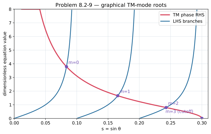
Figure 61 — Problem 8.2-9: graphical TM-mode solution. Positive branches of the left side intersect the reflection-phase curve at the listed roots; the fourth point lies exactly at cutoff.

The book’s count is the smallest integer strictly greater than \(s_c/[\lambda/(2d)]=3\), so

(65)\[\boxed{M_{\rm TM}=4}.\]

Only the first three have \(\gamma>0\); \(m=3\) is marginal at the specified exact cutoff. A plot that omits its endpoint will appear to show only three intersections.

Check. Removing the TM index-squared factor recovers the TE equation; every listed root is on its proper branch and does not exceed cutoff.

Problem 8.3-1 — Rectangular-guide mode count

Brief solution

1. Method. The area mode-count approximation, wavelength-frequency relation, and dimensional checks are used below.

2. Key step.

The square area is \(A=d^2=10^{-2}\ \mathrm{mm^2}=10^{-8}\ \mathrm{m^2}\), so \(d=10^{-4}\ \mathrm m\); \(\mathrm{NA}=0.1\). For one polarization, Eq. (8.3-3) is

\[M_{\rm rectangular}\simeq\frac\pi4M_{\rm slab}^2.\]

This is the two-dimensional analogue of Fig. 8.2-4. The area estimate is not an exact integer count at small \(M\).

3. Answer.

\[\boxed{M_{\rm TE}(\nu)= \pi A\left(\frac{\mathrm{NA}\,\nu}{c_0}\right)^2 =(3.49549\times10^{-27}\ \mathrm{Hz^{-2}})\nu^2}.\]

Indeed, \(M_{\rm slab}\simeq2d\,\mathrm{NA}\,\nu/c_0\), so

Show detailed stepsHide detailed steps

Definitions and setup. The guide is square, and the requested result counts only the TE polarization family.

Mathematical formulas used. The area mode-count approximation, wavelength-frequency relation, and dimensional checks are used below.

Worked derivation.

The square area is \(A=d^2=10^{-2}\ \mathrm{mm^2}=10^{-8}\ \mathrm{m^2}\), so \(d=10^{-4}\ \mathrm m\); \(\mathrm{NA}=0.1\). For one polarization, Eq. (8.3-3) is

(66)\[M_{\rm TE}\simeq\frac\pi4 \left(\frac{2d}{\lambda_0}\right)^2\mathrm{NA}^2, \qquad \lambda_0=\frac{c_0}{\nu}.\]

Substitution gives

(67)\[\boxed{M_{\rm TE}(\nu)= \pi A\left(\frac{\mathrm{NA}\,\nu}{c_0}\right)^2 =(3.49549\times10^{-27}\ \mathrm{Hz^{-2}})\nu^2}.\]

Approximate TE mode count

\(\nu\) (THz)	\(M_{\rm TE}\)
50	8.739
100	34.955
200	139.820
300	314.594
400	559.279

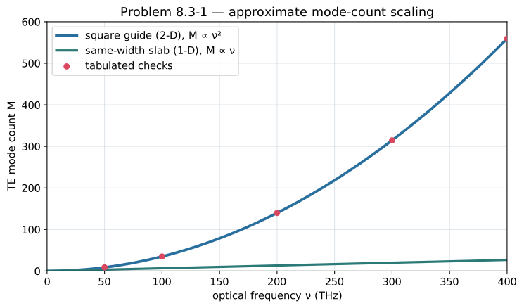
Figure 62 — Problem 8.3-1: TE count versus frequency. A square guide has quadratic growth; the same-width slab comparison is linear. Exact counts would be staircases around these large-mode approximations.

Indeed, \(M_{\rm slab}\simeq2d\,\mathrm{NA}\,\nu/c_0\), so

(68)\[M_{\rm rectangular}\simeq\frac\pi4M_{\rm slab}^2.\]

This is the two-dimensional analogue of Fig. 8.2-4. The area estimate is not an exact integer count at small \(M\).

Check. The coefficient of frequency squared has inverse-hertz-squared units, and substitution at 100 THz gives the tabulated value 34.955.

Problem 8.4-1 — Two-slab coupler

Brief solution

1. Method. Field normalization, exponential and trigonometric integration, and coupled-mode power exchange are used below.

2. Key step.

Each slab has \(d=0.500\ \mu\mathrm m\), \(n_s=1.48\); the medium has \(n=1.46\); the inner-edge gap is \(2a=1.00\ \mu\mathrm m\), so \(a=0.500\ \mu\mathrm m\); and \(\lambda_0=0.850\ \mu\mathrm m\). Put guide 1 in \([-a-d,-a]\) and guide 2 in \([a,a+d]\).

\[P_1(z)=P_1(0)\cos^2(\kappa z),\qquad P_2(z)=P_1(0)\sin^2(\kappa z).\]

Equal powers require \(\kappa L_{3\rm dB}=\pi/4\), hence

3. Answer.

\[\boxed{\kappa=\tfrac12(0.0588) \frac{(7.391983)^2}{10.816010}(0.1111544) =0.0165093\ \mu\mathrm m^{-1} =1.65093\times10^4\ \mathrm m^{-1}}.\]

\[\boxed{L_{3\rm dB}=\frac{\pi}{4\kappa}=47.573\ \mu\mathrm m}.\]

Complete transfer occurs at twice this length, \(L_0=95.146\ \mu\mathrm m\). Increasing the gap decreases the overlap as \(e^{-2\gamma a}\) and must increase both lengths, providing an independent trend check.

Show detailed stepsHide detailed steps

Definitions and setup. The identical isolated TE0 fields are normalized to unity and weakly overlap across the gap, so they are phase matched.

Mathematical formulas used. Field normalization, exponential and trigonometric integration, and coupled-mode power exchange are used below.

Worked derivation.

Each slab has \(d=0.500\ \mu\mathrm m\), \(n_s=1.48\); the medium has \(n=1.46\); the inner-edge gap is \(2a=1.00\ \mu\mathrm m\), so \(a=0.500\ \mu\mathrm m\); and \(\lambda_0=0.850\ \mu\mathrm m\). Put guide 1 in \([-a-d,-a]\) and guide 2 in \([a,a+d]\).

Part (a): evaluate Eq. (8.5-6). Problem 8.2-5 supplies

(69)\[u=0.4108277,\ k_y=1.643311\ \mu\mathrm m^{-1},\quad \gamma=0.715852\ \mu\mathrm m^{-1},\quad \beta=10.816010\ \mu\mathrm m^{-1},\quad N=0.779223\ \mu\mathrm m^{-1/2}.\]

For a guide centered at \(y_c\), use

(70)\[\begin{split}U(y-y_c)=N\begin{cases} \cos[k_y(y-y_c)],&|y-y_c|\le d/2,\\ \cos u\,e^{-\gamma(|y-y_c|-d/2)},&|y-y_c|>d/2. \end{cases}\end{split}\]

Then \(u_1(y)=U[y+(a+d/2)]\) and \(u_2(y)=U[y-(a+d/2)]\). For identical guides,

(71)\[\kappa=\frac12(n_s^2-n^2)\frac{k_0^2}{\beta} \int_a^{a+d}u_1(y)u_2(y)dy.\]

Inside guide 2, guide 1 supplies its exponential tail. With \(x=y-a\),

(72)\[\begin{split}\begin{aligned} I&=N^2\cos u\,e^{-2\gamma a} \int_0^d e^{-\gamma x}\cos[k_y(x-d/2)]dx\\ &=0.1111544. \end{aligned}\end{split}\]

Now \(k_0=2\pi/0.85=7.391983\ \mu\mathrm m^{-1}\) and \(n_s^2-n^2=0.0588000\), so

(73)\[\boxed{\kappa=\tfrac12(0.0588) \frac{(7.391983)^2}{10.816010}(0.1111544) =0.0165093\ \mu\mathrm m^{-1} =1.65093\times10^4\ \mathrm m^{-1}}.\]

The normalized overlap is dimensionless, leaving the correct inverse-length unit from \(k_0^2/\beta\).

Part (b): 3-dB length. Identical, phase-matched guides obey

(74)\[P_1(z)=P_1(0)\cos^2(\kappa z),\qquad P_2(z)=P_1(0)\sin^2(\kappa z).\]

Equal powers require \(\kappa L_{3\rm dB}=\pi/4\), hence

(75)\[\boxed{L_{3\rm dB}=\frac{\pi}{4\kappa}=47.573\ \mu\mathrm m}.\]

Complete transfer occurs at twice this length, \(L_0=95.146\ \mu\mathrm m\). Increasing the gap decreases the overlap as \(e^{-2\gamma a}\) and must increase both lengths, providing an independent trend check.

Check. At the 3-dB length both squared trigonometric factors are one half; at twice that length all power transfers to guide 2.