Matrix-Optics Reference Tables

This page recreates the four principal summary tables in Gerrard and Burch as Sphinx-native tables. Notation has been regularized and short verification notes have been added. The diagrams are original SVG companions rather than scans of the printed pages.

Ray-transfer matrices

Use the reduced ray vector \(\mathbf r=(y,V)^T=(y,nv)^T\), surface power \(P=(n_2-n_1)/r\), and translation \(T(t,n)=(1,t/n;0,1)\). For a mirror the outgoing index changes sign, so \(P=-2n/r\).

Recreated Table 1 — common ray-transfer matrices

No.	Situation	Matrix	Quick check
1	Translation through thickness \(t\) in index \(n\)	\(\begin{bmatrix}1&t/n\\0&1\end{bmatrix}\)	Heights shear; \(V\) is unchanged.
2	Refraction at one spherical surface	\(\begin{bmatrix}1&0\\-P&1\end{bmatrix}\), \(P=(n_2-n_1)/r\)	Height is continuous.
3	Reflection at one spherical surface	\(\begin{bmatrix}1&0\\2n/r&1\end{bmatrix}\)	Plane mirror: \(r\to\infty\) gives \(I\).
4	Thin lens in air, focal length \(f\)	\(\begin{bmatrix}1&0\\-1/f&1\end{bmatrix}\)	Parallel ray crosses axis after \(f\).
5	Between the principal planes of a lens system	\(\begin{bmatrix}1&0\\-1/f&1\end{bmatrix}\)	Same reduced action as a thin lens.
6	Between the two focal planes	\(\begin{bmatrix}0&f\\-1/f&0\end{bmatrix}\)	Height and angle exchange roles.
7	Imaging between conjugate planes with lateral magnification \(m\)	\(\begin{bmatrix}m&0\\-1/f&1/m\end{bmatrix}\)	\(B=0\); object height alone fixes image height.
8	Afocal system with lateral magnification \(m\)	\(\begin{bmatrix}m&0\\0&1/m\end{bmatrix}\)	\(C=0\); parallel input remains parallel.

Every matrix has determinant one. For a compound system, multiply in reverse order of encounter so the rightmost factor acts first.

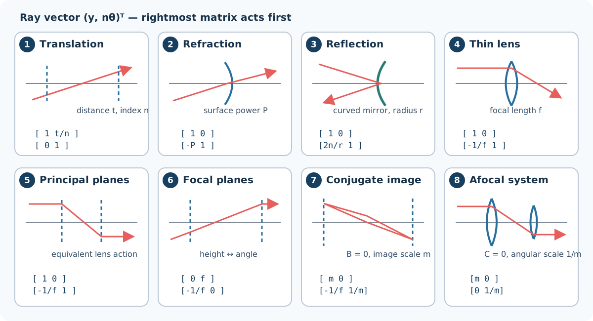
Optical meaning of the eight matrices in the recreated ray-transfer table.

Resonator and Gaussian-beam relations

Let \(M=(A,B;C,D)\) be a real unimodular round-trip matrix and define \(s=(A+D)/2\).

Recreated Table 2a — eigenvalue and stability summary

Regime	Criterion	Eigenvalues	Interpretation
Positive unstable branch	\(s>1\)	\(\lambda_\pm=e^{\pm\tau}\), \(\cosh\tau=s\)	One eigenray expands while its reciprocal contracts.
Negative unstable branch	\(s<-1\)	\(\lambda_\pm=-e^{\pm\tau}\), \(\cosh\tau=-s\)	Expansion/contraction plus parity reversal.
Stable	\(|s|<1\)	\(\lambda_\pm=e^{\pm i\theta}\), \(\cos\theta=s\)	Bounded ray orbit and confined Gaussian eigenmode.
Marginal	\(|s|=1\)	Repeated \(+1\) or \(-1\)	Stability boundary; diffraction/apertures decide behavior.

For the unstable branches, the real eigenvector curvature may be written

\[R=\frac{\lambda-D}{C}, \qquad \frac1R=\frac{\lambda-A}{B}.\]

For the stable branch, choose the fixed point with the physical imaginary sign:

\[q=\frac{A-D}{2C}+i\frac{\sin\theta}{C}, \qquad \frac1q=\frac{D-A}{2B}+i\frac{\sin\theta}{B}.\]

With the book’s convention \(1/q=1/R+i\lambda/(\pi w^2)\), the associated beam data are:

Recreated Table 2b — Gaussian eigenbeam parameters

Parameter	Formula at the reference plane	Interpretation
Wavefront curvature	\(R=2B/(D-A)\)	Infinite when \(A=D\).
Spot radius	\(w^2=\lambda B/(\pi\sin\theta)\)	Select the eigenvalue branch giving \(w^2>0\).
Neck location	\(z=(A-D)/(2C)\)	Signed distance from the reference plane.
Neck radius	\(w_0^2=-\lambda\sin\theta/(\pi C)\)	Physical branch again requires positivity.
Confocal parameter	\(z_0=-\sin\theta/C=\pi w_0^2/\lambda\)	Half the usual confocal length under this notation.
Mode discrimination warning	Geometrical stability alone is insufficient.	Aperture loss and gain profile select transverse modes.

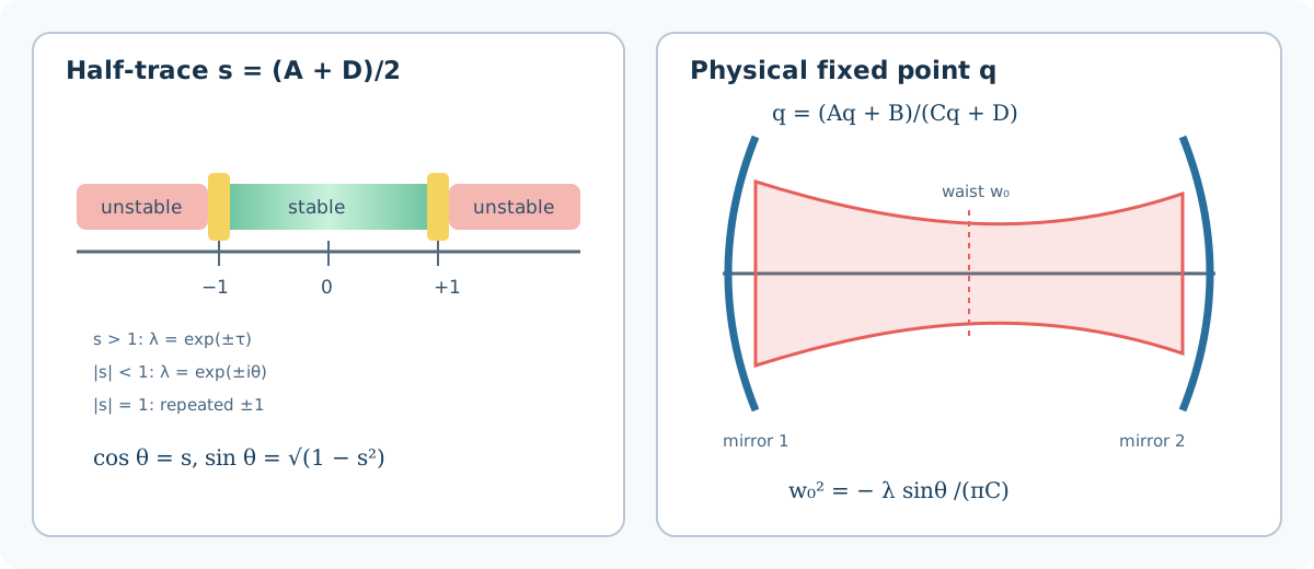
The half-trace classifies the matrix; the physical fixed point supplies the Gaussian eigenmode.

Mueller matrices

Use Stokes order \((I,Q,U,V)^T\), \(C_2=\cos2\theta\), \(S_2=\sin2\theta\), \(\beta=\cos\delta\), and \(\mu=\sin\delta\).

Recreated Table 3 — ideal Mueller elements

Device	Mueller matrix	Special cases
Linear polarizer at \(\theta\)	\(\dfrac12\begin{bmatrix} 1&C_2&S_2&0\\C_2&C_2^2&C_2S_2&0\\ S_2&C_2S_2&S_2^2&0\\0&0&0&0 \end{bmatrix}\)	\(\theta=0\) passes \(+Q\); \(\theta=\pi/2\) passes \(-Q\).
Linear retarder, retardance \(\delta\), fast axis \(\theta\)	\(\begin{bmatrix} 1&0&0&0\\ 0&C_2^2+S_2^2\beta&C_2S_2(1-\beta)&-S_2\mu\\ 0&C_2S_2(1-\beta)&S_2^2+C_2^2\beta&C_2\mu\\ 0&S_2\mu&-C_2\mu&\beta \end{bmatrix}\)	Quarter wave: \(\delta=\pi/2\); half wave: \(\delta=\pi\).
Quarter-wave retarder, fast axis horizontal	\(\begin{bmatrix}1&0&0&0\\0&1&0&0\\0&0&0&1\\0&0&-1&0\end{bmatrix}\)	Interchanges \(U\) and \(V\) with the convention’s signs.
Half-wave retarder, fast axis horizontal	\(\operatorname{diag}(1,1,-1,-1)\)	Reverses the \(U,V\) components.
Rotation of axes through \(\theta\)	\(R_M(\theta)=\begin{bmatrix} 1&0&0&0\\0&C_2&S_2&0\\0&-S_2&C_2&0\\0&0&0&1 \end{bmatrix}\)	Rotates the linear Stokes pair by \(2\theta\).

A device rotated from its tabulated zero-angle form transforms as

\[\boxed{M(\theta+\phi)=R_M(-\theta)M(\phi)R_M(\theta)}.\]

Jones matrices

Use \(c=\cos\theta\), \(s=\sin\theta\). Overall nonzero complex scalars are physically irrelevant unless absolute transmission or phase is being compared.

Recreated Table 4 — ideal Jones elements

Device	Jones matrix	Special cases
Linear polarizer at \(\theta\)	\(\begin{bmatrix}c^2&cs\\cs&s^2\end{bmatrix}\)	\(\theta=0\): \(\operatorname{diag}(1,0)\); \(\theta=\pi/2\): \(\operatorname{diag}(0,1)\).
Linear retarder, retardance \(\delta\), fast axis \(\theta\)	\(\begin{bmatrix} c^2+s^2e^{-i\delta}&cs(1-e^{-i\delta})\\ cs(1-e^{-i\delta})&s^2+c^2e^{-i\delta} \end{bmatrix}\)	At \(\theta=0\): \(\operatorname{diag}(1,e^{-i\delta})\).
Quarter-wave retarder	Set \(\delta=\pi/2\) in the general retarder.	Converts suitable linear states to circular states and conversely.
Half-wave retarder	\(\begin{bmatrix}\cos2\theta&\sin2\theta\\ \sin2\theta&-\cos2\theta\end{bmatrix}\) up to common phase	Rotates a linear polarization direction through twice the plate angle.
Rotation of axes through \(\theta\)	\(R_J(\theta)=\begin{bmatrix}c&s\\-s&c\end{bmatrix}\)	Also represents an ideal circular retarder with the associated angle.

The rotation rule is

\[\boxed{J(\theta+\phi)=R_J(-\theta)J(\phi)R_J(\theta)}.\]

Jones calculus retains complex field phase but applies only to fully polarized light. Mueller calculus propagates measurable Stokes data and also handles partial or unpolarized states.

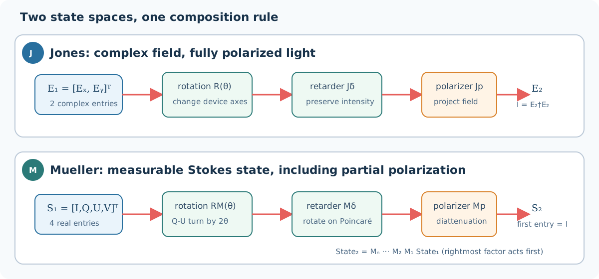
Jones and Mueller products use the same rightmost-first composition rule, but operate on different state spaces.