Chapter 15: Lasers
Source: Saleh and Teich, Fundamentals of Photonics, second edition, Chapter 15.
In-text exercises
Exercise 15.1-1 — Ruby threshold
Brief solution
1. Method. The working uses exponential, logarithmic, and phasor identities and algebraic rearrangement and dimensional checks.
2. Reasoning and answer.
Show detailed steps
Step 1 — Definitions and setup. Symbols are local to this item and follow the chapter convention. Each physical quantity and supplied numerical value is introduced at its first use below; angles are in radians unless a degree symbol is shown, and units are retained through numerical substitution.
Figure 88 — Exercise 15.1-1: Ruby threshold. The diagram identifies the input quantities, physical operation, requested result, variable meanings, and an independent verification route. Every symbol in the variable strip is labeled on the model itself.
Step 2 — Mathematical formulas used. The working uses exponential, logarithmic, and phasor identities and algebraic rearrangement and dimensional checks.
Step 3 — Worked derivation. The calculation is kept in symbolic form until the governing relation has been rearranged for the requested quantity.
Detailed step 1. Thermal absorption gives \(\sigma_0=0.2/(1.58\times10^{19})= \boxed{1.27\times10^{-20}\ \mathrm{cm^2}}\).
Detailed step 2. Mirror loss is \(\alpha_r=-\ln(R_1R_2)/(2d)\); threshold inversion is \(\boxed{N_t=\alpha_r/\sigma_0}\) and threshold excited population follows from \(N=N_2-N_1=2N_2-N_a\) for this three-level transition.
Step 4 — State the numbered result. The principal result obtained in the working is
Step 5 — Check. Equation (1) can be checked by substituting it back into the preceding governing relation and reversing the algebraic steps. Check that dimensions agree term by term, then test the simplest symmetry or limiting case for the expected sign and scale. Repeat the substitution with unrounded intermediate values and retain the displayed units; the final unit must have the requested dimension.
Exercise 15.2-1 — Gas-laser oscillation band
Brief solution
1. Method. The working uses integration identities, exponential, logarithmic, and phasor identities, and algebraic rearrangement and dimensional checks.
2. Reasoning and answer.
Show detailed steps
Step 1 — Definitions and setup. Symbols are local to this item and follow the chapter convention. Each physical quantity and supplied numerical value is introduced at its first use below; angles are in radians unless a degree symbol is shown, and units are retained through numerical substitution.
Figure 89 — Exercise 15.2-1: Gas-laser oscillation band. The diagram identifies the input quantities, physical operation, requested result, variable meanings, and an independent verification route. Every symbol in the variable strip is labeled on the model itself.
Step 2 — Mathematical formulas used. The working uses integration identities, exponential, logarithmic, and phasor identities, and algebraic rearrangement and dimensional checks.
Step 3 — Worked derivation. The calculation is kept in symbolic form until the governing relation has been rearranged for the requested quantity.
Detailed step 1. Set Gaussian gain equal to loss at both band edges: \(\boxed{B=\Delta\nu_D \sqrt{\ln(\gamma_0/\alpha_r)/\ln2}}\).
Detailed step 2. Divide by cavity FSR \(c/(2nd)\) and count the integer modes whose frequencies lie inside this band; the given He–Ne parameters supply the requested count.
Step 4 — State the numbered result. The principal result obtained in the working is
Step 5 — Check. Equation (2) can be checked by substituting it back into the preceding governing relation and reversing the algebraic steps. Differentiation of an antiderivative, or normalization of a definite integral, checks the integration step.
Exercise 15.4-1 — Four-level population equation
Brief solution
1. Method. Write a rate balance for each laser level, use adiabatic elimination for the short-lived lower level, and then use the textbook relation
2. Key step.
The missing factor of 2 is physical, not algebraic. In a three-level laser, one stimulated emission event changes \(N_2\mapsto N_2-1\) and \(N_1\mapsto N_1+1\), so \(N_2-N_1\) initially falls by two. In the four-level laser, the atom added to level 1 immediately decays to level 0; that cleanup raises \(N_2-N_1\) by one again. The net change observed on the laser timescale is therefore only \(\Delta N=-1\) per generated photon.
3. Answer.
Show detailed steps
Step 1 — Definitions and setup. Use the four-level scheme of Fig. 14.2-6: the pump transfers atoms from level 0 through the short-lived level 3 into the upper laser level 2 at the effective rate \(R\). The laser transition is \(2\rightarrow1\), and the lower laser level empties to level 0 with \(\tau_1\ll t_{sp}\). Here \(N_i\) is the population density of level \(i\), \(N=N_2-N_1\) is the population difference, \(W_i\) is the induced-transition probability per atom, \(n\) is the resonator photon density, \(N_t\) is the threshold population difference, and \(t_p\) is the photon lifetime. As in the surrounding textbook derivation, assume that \(R\) is independent of \(N\).
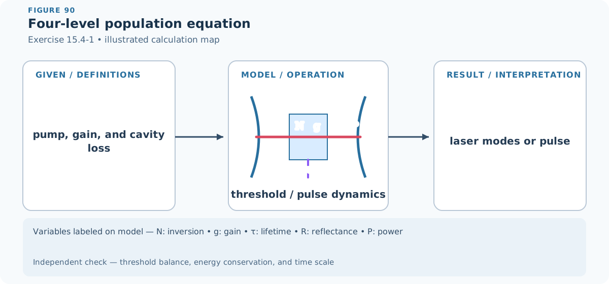
Figure 90 — Exercise 15.4-1: Four-level population equation. The lower laser level does not retain the atom delivered by a stimulated transition. Its rapid \(1\rightarrow0\) decay changes the initial inversion change of \(-2\) into a net slow-timescale change of \(-1\).
Step 2 — Mathematical formulas used. Write a rate balance for each laser level, use adiabatic elimination for the short-lived lower level, and then use the textbook relation
from Eq. (15.4-2). The algebra and units can be checked with algebraic rearrangement and dimensional checks.
Step 3 — Worked derivation. Start with separate upper- and lower-level balances. Pumping adds atoms to level 2; spontaneous decay and net induced transitions remove them. The same two processes feed level 1, which rapidly empties to level 0:
Because \(\tau_1\) is the shortest timescale, level 1 follows the other variables almost instantaneously. Set \(dN_1/dt\simeq0\) in the second equation to obtain
Thus \(N=N_2-N_1\simeq N_2\) and, on timescales long compared with \(\tau_1\), \(dN/dt\simeq dN_2/dt\). The first equation in (4) therefore reduces to
For the assumed population-independent pump, Eq. (14.2-13) gives the small-signal population difference \(N_0=Rt_{sp}\). Substitute this definition and (3) into (6):
The missing factor of 2 is physical, not algebraic. In a three-level laser, one stimulated emission event changes \(N_2\mapsto N_2-1\) and \(N_1\mapsto N_1+1\), so \(N_2-N_1\) initially falls by two. In the four-level laser, the atom added to level 1 immediately decays to level 0; that cleanup raises \(N_2-N_1\) by one again. The net change observed on the laser timescale is therefore only \(\Delta N=-1\) per generated photon.
Step 4 — State the numbered result. The principal result obtained in the working is
Step 5 — Check. With no resonator field (\(n=0\)), (8) gives \(N(t)=N_0+[N(0)-N_0]e^{-t/t_{sp}}\), so the unilluminated inversion tends to \(N_0\) with the correct lifetime. During nonzero steady lasing, Eq. (15.4-3) requires \(N=N_t\); the result above then gives
which is twice the three-level value following Eq. (15.4-6), exactly as expected when the factor of 2 is absent. Finally, every term in (8) has units of population density per unit time.
Exercise 15.4-2 — Q-switched ruby pulse
Brief solution
1. Method. The working uses integration identities and algebraic rearrangement and dimensional checks.
2. Reasoning and answer.
Show detailed steps
Step 1 — Definitions and setup. Symbols are local to this item and follow the chapter convention. Each physical quantity and supplied numerical value is introduced at its first use below; angles are in radians unless a degree symbol is shown, and units are retained through numerical substitution.
Figure 91 — Exercise 15.4-2: Q-switched ruby pulse. The diagram identifies the input quantities, physical operation, requested result, variable meanings, and an independent verification route. Every symbol in the variable strip is labeled on the model itself.
Step 2 — Mathematical formulas used. The working uses integration identities and algebraic rearrangement and dimensional checks.
Step 3 — Worked derivation. The calculation is kept in symbolic form until the governing relation has been rearranged for the requested quantity.
Detailed step 1. For \(N_i/N_t=6\),
Detailed step 2. read the normalized peak,
Detailed step 3. duration,
Detailed step 4. and extracted population from Fig.
Detailed step 5. 15.4-8; dimensionalize time by \(t_p\),
Detailed step 6. photon density by \(N_t\),
Detailed step 7. power by \(h\nu V/t_p\),
Detailed step 8. and energy by \(h\nu V(N_i-N_f)/2\).
Detailed step 9. Recording the graph-read coordinates avoids false precision from the scanned plot.
Step 4 — State the numbered result. The principal result obtained in the working is
Step 5 — Check. Equation (10) can be checked by substituting it back into the preceding governing relation and reversing the algebraic steps. Differentiation of an antiderivative, or normalization of a definite integral, checks the integration step. Repeat the substitution with unrounded intermediate values and retain the displayed units; the final unit must have the requested dimension.
Exercise 15.4-3 — Mode-locking computation
Brief solution
1. Method. The working uses expectation, variance, and probability identities, integration identities, and exponential, logarithmic, and phasor identities.
Show detailed steps
Step 1 — Definitions and setup. Symbols are local to this item and follow the chapter convention. Each physical quantity and supplied numerical value is introduced at its first use below; angles are in radians unless a degree symbol is shown, and units are retained through numerical substitution.
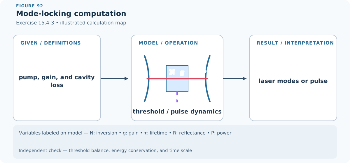
Figure 92 — Exercise 15.4-3: Mode-locking computation. The diagram identifies the input quantities, physical operation, requested result, variable meanings, and an independent verification route. Every symbol in the variable strip is labeled on the model itself.
Step 2 — Mathematical formulas used. The working uses expectation, variance, and probability identities, integration identities, and exponential, logarithmic, and phasor identities.
Step 3 — Worked derivation. The calculation is kept in symbolic form until the governing relation has been rearranged for the requested quantity.
Detailed step 1. Evaluate \(A(t)=\sum_{q=-5}^{5}A_qe^{j2\pi q\nu_Ft}\) on one period.
Detailed step 2. Equal phases give the squared Dirichlet kernel;
Detailed step 3. Gaussian magnitudes give a Gaussian-like pulse; random phases give irregular low-contrast fluctuations.
Detailed step 4. Normalize each case by \(\sum|A_q|^2\) for a fair power comparison.
End-of-chapter problems
Step 4 — State the numbered result. The principal result obtained in the working is
Step 5 — Check. Equation (11) can be checked by substituting it back into the preceding governing relation and reversing the algebraic steps. For a probability result, verify the zero-to-one bounds; when a full distribution is present, also verify normalization and nonnegative variance.
Problem 15.2-2 — Argon longitudinal modes
Brief solution
1. Method. The working uses algebraic rearrangement and dimensional checks.
2. Reasoning and answer.
Show detailed steps
Definitions and setup. Symbols are local to this item and follow the chapter convention. Each physical quantity and supplied numerical value is introduced at its first use below; angles are in radians unless a degree symbol is shown, and units are retained through numerical substitution.
Mathematical formulas used. The working uses algebraic rearrangement and dimensional checks.
Worked derivation. The calculation is kept in symbolic form until the governing relation has been rearranged for the requested quantity.
Detailed step 1. \(\nu_F=c/(2d)=149.9\) MHz.
Detailed step 2. Half-peak loss permits the Doppler FWHM \(B=3.5\) GHz,
Detailed step 3. about \(\boxed{23}\) longitudinal spacings.
Detailed step 4. Single mode requires \(c/(2d)>B\),
Detailed step 5. so \(d<4.28\) cm for Ar+ and \(d<2.50\) m for the 60-MHz CO2 line.
Numbered result. The principal result obtained in the working is
Check. Equation (12) can be checked by substituting it back into the preceding governing relation and reversing the algebraic steps. Check that dimensions agree term by term, then test the simplest symmetry or limiting case for the expected sign and scale. Repeat the substitution with unrounded intermediate values and retain the displayed units; the final unit must have the requested dimension.
Problem 15.2-3 — Length range for one/two modes
Brief solution
1. Method. The working uses exponential, logarithmic, and phasor identities and algebraic rearrangement and dimensional checks.
2. Reasoning and answer.
Show detailed steps
Definitions and setup. Symbols are local to this item and follow the chapter convention. Each physical quantity and supplied numerical value is introduced at its first use below; angles are in radians unless a degree symbol is shown, and units are retained through numerical substitution.
Mathematical formulas used. The working uses exponential, logarithmic, and phasor identities and algebraic rearrangement and dimensional checks.
Worked derivation. The calculation is kept in symbolic form until the governing relation has been rearranged for the requested quantity.
Detailed step 1. Compute \(\alpha_r=-\ln(0.97)/(2d)\),
Detailed step 2. then \(B(d)=\Delta\nu_D\sqrt{\ln(\gamma_0/\alpha_r)/\ln2}\).
Detailed step 3. The required lengths satisfy \(1\leq B/[c/(2d)]<3\); solve the two equality boundaries numerically and exclude lengths for which \(\gamma_0\leq\alpha_r\).
Numbered result. The principal result obtained in the working is
Check. Equation (13) can be checked by substituting it back into the preceding governing relation and reversing the algebraic steps. Check that dimensions agree term by term, then test the simplest symmetry or limiting case for the expected sign and scale.
Problem 15.2-4 — Etalon selector
Brief solution
1. Method. The working uses Fourier-transform and convolution identities and algebraic rearrangement and dimensional checks.
2. Reasoning and answer.
Show detailed steps
Definitions and setup. Symbols are local to this item and follow the chapter convention. Each physical quantity and supplied numerical value is introduced at its first use below; angles are in radians unless a degree symbol is shown, and units are retained through numerical substitution.
Mathematical formulas used. The working uses Fourier-transform and convolution identities and algebraic rearrangement and dimensional checks.
Worked derivation. The calculation is kept in symbolic form until the governing relation has been rearranged for the requested quantity.
Detailed step 1. Choose etalon FSR \(c/(2d_e)>1.5\) GHz (for example \(d_e<10\) cm) and linewidth \(\nu_{F,e}/\mathcal F\) narrower than the laser’s 300-MHz longitudinal spacing; \(d_e=5\) cm and \(\mathcal F>10\) is a workable pair.
Detailed step 2. Intracavity placement suppresses unwanted modes before gain saturation and is therefore superior.
Numbered result. The principal result obtained in the working is
Check. Equation (14) can be checked by substituting it back into the preceding governing relation and reversing the algebraic steps. Transform dimensions and the expected even/odd or conjugate symmetry provide an independent check on signs and scale factors. Repeat the substitution with unrounded intermediate values and retain the displayed units; the final unit must have the requested dimension.
Problem 15.2-5 — Multimode He–Ne power
Brief solution
1. Method. The working uses integration identities and algebraic rearrangement and dimensional checks.
2. Reasoning and answer.
Show detailed steps
Definitions and setup. Symbols are local to this item and follow the chapter convention. Each physical quantity and supplied numerical value is introduced at its first use below; angles are in radians unless a degree symbol is shown, and units are retained through numerical substitution.
Mathematical formulas used. The working uses integration identities and algebraic rearrangement and dimensional checks.
Worked derivation. The calculation is kept in symbolic form until the governing relation has been rearranged for the requested quantity.
Detailed step 1. At gain/loss ratio two,
Detailed step 2. the permitted Gaussian band is one FWHM;
Detailed step 3. FSR is \(c/(0.6)=499.7\) MHz,
Detailed step 4. giving roughly three modes.
Detailed step 5. Centering one mode makes its saturated gain competition strongest; a first equal-sharing estimate is \(\boxed{50/3\simeq16.7\ \mathrm{mW}}\),
Detailed step 6. refined by weighting each mode with its Gaussian excess gain.
Numbered result. The principal result obtained in the working is
Check. Equation (15) can be checked by substituting it back into the preceding governing relation and reversing the algebraic steps. Differentiation of an antiderivative, or normalization of a definite integral, checks the integration step. Repeat the substitution with unrounded intermediate values and retain the displayed units; the final unit must have the requested dimension.
Problem 15.2-6 — Single-mode output
Brief solution
1. Method. The working uses exponential, logarithmic, and phasor identities and algebraic rearrangement and dimensional checks.
2. Reasoning and answer.
Show detailed steps
Definitions and setup. Symbols are local to this item and follow the chapter convention. Each physical quantity and supplied numerical value is introduced at its first use below; angles are in radians unless a degree symbol is shown, and units are retained through numerical substitution.
Mathematical formulas used. The working uses exponential, logarithmic, and phasor identities and algebraic rearrangement and dimensional checks.
Worked derivation. The calculation is kept in symbolic form until the governing relation has been rearranged for the requested quantity.
Detailed step 1. \(\alpha_{m1}=-\ln0.99/(2d)\), \(\alpha_{m2}=0\),
Detailed step 2. and \(\alpha_r=\alpha_{m1}\).
Detailed step 3. Then \(t_p=n/(c\alpha_r)\) and intracavity steady flux is \(\phi_s(\gamma_0/\alpha_r-1)\); multiply by output transmission,
Detailed step 4. photon energy,
Detailed step 5. and \(1\ \mathrm{mm^2}\) area for \(P_o\).
Numbered result. The principal result obtained in the working is
Check. Equation (16) can be checked by substituting it back into the preceding governing relation and reversing the algebraic steps. Check that dimensions agree term by term, then test the simplest symmetry or limiting case for the expected sign and scale. Repeat the substitution with unrounded intermediate values and retain the displayed units; the final unit must have the requested dimension.
Problem 15.2-7 — Reading a passive cavity trace
Brief solution
1. Method. The working uses algebraic rearrangement and dimensional checks.
2. Reasoning and answer.
Show detailed steps
Definitions and setup. Symbols are local to this item and follow the chapter convention. Each physical quantity and supplied numerical value is introduced at its first use below; angles are in radians unless a degree symbol is shown, and units are retained through numerical substitution.
Mathematical formulas used. The working uses algebraic rearrangement and dimensional checks.
Worked derivation. The calculation is kept in symbolic form until the governing relation has been rearranged for the requested quantity.
Detailed step 1. Read peak spacing \(\nu_F\) and FWHM \(\delta\nu\) from the supplied plot.
Detailed step 2. Then \(d=c/(2\nu_F)\), \(t_p=1/(2\pi\delta\nu)\),
Detailed step 3. and \(\gamma_t=1/(ct_p)\).
Detailed step 4. Subthreshold pumping narrows and raises peaks symmetrically around \(5\times10^{14}\) Hz but cannot make their width zero.
Numbered result. The principal result obtained in the working is
Check. Equation (17) can be checked by substituting it back into the preceding governing relation and reversing the algebraic steps. Check that dimensions agree term by term, then test the simplest symmetry or limiting case for the expected sign and scale.
Problem 15.2-8 — Four-level rate equations
Brief solution
1. Method. The working uses algebraic rearrangement and dimensional checks.
2. Reasoning and answer.
Show detailed steps
Definitions and setup. Symbols are local to this item and follow the chapter convention. Each physical quantity and supplied numerical value is introduced at its first use below; angles are in radians unless a degree symbol is shown, and units are retained through numerical substitution.
Mathematical formulas used. The working uses algebraic rearrangement and dimensional checks.
Worked derivation. The calculation is kept in symbolic form until the governing relation has been rearranged for the requested quantity.
Detailed step 1. Write level equations with pump relaxation and stimulated term \(\sigma cn(N_2-N_1)\); subtraction gives \(\dot N=(N_0-N)/T_s-\sigma cnN\) and \(\dot n=\sigma cnN-n/t_p+N_2/t_{sp}\).
Detailed step 2. Above threshold, \(N\simeq N_t=1/(\sigma ct_p)\) and the excess pump fixes steady \(n\).
Numbered result. The principal result obtained in the working is
Check. Equation (18) can be checked by substituting it back into the preceding governing relation and reversing the algebraic steps. Check that dimensions agree term by term, then test the simplest symmetry or limiting case for the expected sign and scale.
Problem 15.3-1 — Yb:YAG design
Brief solution
1. Method. The working uses exponential, logarithmic, and phasor identities and algebraic rearrangement and dimensional checks.
2. Reasoning and answer.
Show detailed steps
Definitions and setup. Symbols are local to this item and follow the chapter convention. Each physical quantity and supplied numerical value is introduced at its first use below; angles are in radians unless a degree symbol is shown, and units are retained through numerical substitution.
Mathematical formulas used. The working uses exponential, logarithmic, and phasor identities and algebraic rearrangement and dimensional checks.
Worked derivation. The calculation is kept in symbolic form until the governing relation has been rearranged for the requested quantity.
Detailed step 1. Convert the pump energy by \(\lambda=hc/E\) and its endpoint energies to obtain band width in nanometres.
Detailed step 2. Thermal populations give \(\alpha=-\sigma_0N\); the 6-cm cavity has \(\alpha_r=-\ln0.8/(12\ \mathrm{cm})\), \(t_p=n/(c\alpha_r)\),
Detailed step 3. and \(N_t=\alpha_r/\sigma_0\).
Detailed step 4. A small pump- laser energy defect improves quantum efficiency;
Detailed step 5. YVO4 changes host index,
Detailed step 6. cross section,
Detailed step 7. lifetime,
Detailed step 8. thermal conductivity,
Detailed step 9. and hence threshold/output.
Numbered result. The principal result obtained in the working is
Check. Equation (19) can be checked by substituting it back into the preceding governing relation and reversing the algebraic steps. Check that dimensions agree term by term, then test the simplest symmetry or limiting case for the expected sign and scale. Repeat the substitution with unrounded intermediate values and retain the displayed units; the final unit must have the requested dimension.
Problem 15.3-2 — Ar+ threshold
Brief solution
1. Method. The working uses exponential, logarithmic, and phasor identities and algebraic rearrangement and dimensional checks.
2. Reasoning and answer.
Show detailed steps
Definitions and setup. Symbols are local to this item and follow the chapter convention. Each physical quantity and supplied numerical value is introduced at its first use below; angles are in radians unless a degree symbol is shown, and units are retained through numerical substitution.
Mathematical formulas used. The working uses exponential, logarithmic, and phasor identities and algebraic rearrangement and dimensional checks.
Worked derivation. The calculation is kept in symbolic form until the governing relation has been rearranged for the requested quantity.
Detailed step 1. \(t_p=[c(-\ln0.98/2d)]^{-1}\).
Detailed step 2. Convert 0.003-nm linewidth to frequency,
Detailed step 3. use lifetime/lineshape to find \(\sigma_0\),
Detailed step 4. then \(\boxed{N_t=1/(\sigma_0ct_p)}\); the mode diameter affects total excited ion number,
Detailed step 5. not density threshold.
Numbered result. The principal result obtained in the working is
Check. Equation (20) can be checked by substituting it back into the preceding governing relation and reversing the algebraic steps. Check that dimensions agree term by term, then test the simplest symmetry or limiting case for the expected sign and scale. Repeat the substitution with unrounded intermediate values and retain the displayed units; the final unit must have the requested dimension.
Problem 15.3-3 — EUV spontaneous lifetime
Brief solution
1. Method. The working uses algebraic rearrangement and dimensional checks.
2. Reasoning and answer.
Show detailed steps
Definitions and setup. Symbols are local to this item and follow the chapter convention. Each physical quantity and supplied numerical value is introduced at its first use below; angles are in radians unless a degree symbol is shown, and units are retained through numerical substitution.
Mathematical formulas used. The working uses algebraic rearrangement and dimensional checks.
Worked derivation. The calculation is kept in symbolic form until the governing relation has been rearranged for the requested quantity.
Detailed step 1. For equal line strength,
Detailed step 2. Einstein \(A\propto\nu^3\),
Detailed step 3. so \(t_{sp}\propto\lambda^3\).
Detailed step 4. Thus \(\boxed{t_{EUV}=10\ \mathrm{ns}(18.2/500)^3=0.482\ \mathrm{ps}}\),
Detailed step 5. of the same scale as the tabulated value.
Numbered result. The principal result obtained in the working is
Check. Equation (21) can be checked by substituting it back into the preceding governing relation and reversing the algebraic steps. Check that dimensions agree term by term, then test the simplest symmetry or limiting case for the expected sign and scale. Repeat the substitution with unrounded intermediate values and retain the displayed units; the final unit must have the requested dimension.
Problem 15.4-4 — Gain-switch transients
Brief solution
1. Method. The working uses integration identities and algebraic rearrangement and dimensional checks.
2. Reasoning and answer.
Show detailed steps
Definitions and setup. Symbols are local to this item and follow the chapter convention. Each physical quantity and supplied numerical value is introduced at its first use below; angles are in radians unless a degree symbol is shown, and units are retained through numerical substitution.
Mathematical formulas used. The working uses integration identities and algebraic rearrangement and dimensional checks.
Worked derivation. The calculation is kept in symbolic form until the governing relation has been rearranged for the requested quantity.
Detailed step 1. The stated substitutions directly produce \(X'=-X+XY\), \(Y'=a(Y_0-Y)-2XY\).
Detailed step 2. Integrate with an adaptive ODE solver for the three \(a\) values and define switching time by 10–90% photon density.
Detailed step 3. The \(10^{-5}\) seed represents spontaneous emission; small \(a\) gives relaxation spiking,
Detailed step 4. large \(a\) follows pump rapidly.
Numbered result. The principal result obtained in the working is
Check. Equation (22) can be checked by substituting it back into the preceding governing relation and reversing the algebraic steps. Differentiation of an antiderivative, or normalization of a definite integral, checks the integration step.
Problem 15.4-5 — Q-switched ruby energetics
Brief solution
1. Method. The working uses integration identities, exponential, logarithmic, and phasor identities, and algebraic rearrangement and dimensional checks.
2. Reasoning and answer.
Show detailed steps
Definitions and setup. Symbols are local to this item and follow the chapter convention. Each physical quantity and supplied numerical value is introduced at its first use below; angles are in radians unless a degree symbol is shown, and units are retained through numerical substitution.
Mathematical formulas used. The working uses integration identities, exponential, logarithmic, and phasor identities, and algebraic rearrangement and dimensional checks.
Worked derivation. The calculation is kept in symbolic form until the governing relation has been rearranged for the requested quantity.
Detailed step 1. Maintenance pump is \(N_2V(hc/450\mathrm{nm})/t_{sp}\); spontaneous power is \(N_2V(hc/694.3\mathrm{nm})/t_{sp}\).
Detailed step 2. Compute \(N_t=-\ln(R_1R_2)/(2d_r\sigma)\) and use Q-switch invariants to solve \(N_f-N_t\ln N_f=N_i-N_t\ln N_i\); extracted pulse energy is \(h\nu V(N_i-N_f)/2\),
Detailed step 3. with peak/duration from the normalized rate solution.
Numbered result. The principal result obtained in the working is
Check. Equation (23) can be checked by substituting it back into the preceding governing relation and reversing the algebraic steps. Differentiation of an antiderivative, or normalization of a definite integral, checks the integration step. Repeat the substitution with unrounded intermediate values and retain the displayed units; the final unit must have the requested dimension.
Problem 15.4-6 — Cavity dumping timeline
Brief solution
1. Method. The working uses the physical definitions stated in the item; no separate calculus or algebraic identity is required for this qualitative comparison.
Show detailed steps
Definitions and setup. Symbols are local to this item and follow the chapter convention. Each physical quantity and supplied numerical value is introduced at its first use below; angles are in radians unless a degree symbol is shown, and units are retained through numerical substitution.
Mathematical formulas used. The working uses the physical definitions stated in the item; no separate calculus or algebraic identity is required for this qualitative comparison.
Worked derivation. The calculation is kept in symbolic form until the governing relation has been rearranged for the requested quantity.
Detailed step 1. During high-Q storage,
Detailed step 2. threshold is low, \(N\) clamps,
Detailed step 3. internal photons rise,
Detailed step 4. and external output is small.
Detailed step 5. Opening the dump raises threshold abruptly,
Detailed step 6. empties internal photons as one large external pulse,
Detailed step 7. and lets \(N\) recover under pumping; repeat this four-trace sequence for cycle two.
Check. For a qualitative conclusion, test every absolute statement against the stated assumptions and at least one limiting case or counterexample.
Problem 15.4-7 — Lorentzian mode locking
Brief solution
1. Method. The working uses stationary-value condition, Fourier-transform and convolution identities, and exponential, logarithmic, and phasor identities.
Show detailed steps
Definitions and setup. Symbols are local to this item and follow the chapter convention. Each physical quantity and supplied numerical value is introduced at its first use below; angles are in radians unless a degree symbol is shown, and units are retained through numerical substitution.
Mathematical formulas used. The working uses stationary-value condition, Fourier-transform and convolution identities, and exponential, logarithmic, and phasor identities.
Worked derivation. The calculation is kept in symbolic form until the governing relation has been rearranged for the requested quantity.
Detailed step 1. The Fourier series of Lorentzian modal amplitudes is a periodic exponential pulse.
Detailed step 2. Parseval gives mean power \(\sum|A_q|^2\); coherent summation gives peak \(|\sum A_q|^2\); solving the exponential intensity at half maximum gives FWHM proportional to \(1/\Delta\nu\).
Detailed step 3. Evaluating the standard Lorentzian sums supplies the book’s closed constants.
Check. Transform dimensions and the expected even/odd or conjugate symmetry provide an independent check on signs and scale factors.
Problem 15.4-8 — Intracavity second harmonic
Brief solution
1. Method. The working uses algebraic rearrangement and dimensional checks.
2. Reasoning and answer.
Show detailed steps
Definitions and setup. Symbols are local to this item and follow the chapter convention. Each physical quantity and supplied numerical value is introduced at its first use below; angles are in radians unless a degree symbol is shown, and units are retained through numerical substitution.
Mathematical formulas used. The working uses algebraic rearrangement and dimensional checks.
Worked derivation. The calculation is kept in symbolic form until the governing relation has been rearranged for the requested quantity.
Detailed step 1. Two fundamental photons make one harmonic: \(\dot n=\epsilon n-n/t_p-2\zeta n^2\) and \(\dot n_2=\zeta n^2-n_2/t_{p2}\).
Detailed step 2. The nonzero steady solution is \(\boxed{n=(\epsilon-1/t_p)/(2\zeta)}\) and \(\boxed{n_2=\zeta t_{p2}n^2}\) above threshold.
Numbered result. The principal result obtained in the working is
Check. Equation (24) can be checked by substituting it back into the preceding governing relation and reversing the algebraic steps. Check that dimensions agree term by term, then test the simplest symmetry or limiting case for the expected sign and scale.