Chapter 2: Wave Optics
Source: Saleh and Teich, Fundamentals of Photonics, second edition, Chapter 2. The time convention is the one used by the text.
In-text exercises
Exercise 2.2-1 — Fresnel-approximation region
Brief solution
1. Method. The working uses algebraic rearrangement and dimensional checks.
2. Reasoning and answer.
Show detailed steps
Step 1 — Definitions and setup. Symbols are local to this item and follow the chapter convention. Each physical quantity and supplied numerical value is introduced at its first use below; angles are in radians unless a degree symbol is shown, and units are retained through numerical substitution.
Figure 17 — Exercise 2.2-1: Fresnel-approximation region. The diagram identifies the input quantities, physical operation, requested result, variable meanings, and an independent verification route. Every symbol in the variable strip is labeled on the model itself.
Step 2 — Mathematical formulas used. The working uses algebraic rearrangement and dimensional checks.
Step 3 — Worked derivation. The calculation is kept in symbolic form until the governing relation has been rearranged for the requested quantity.
Detailed step 1. At the usual boundary estimate \(a^4=4z^3\lambda\),
Detailed step 2. with \(z=1\ \mathrm m\) and \(\lambda=633\ \mathrm{nm}\), \(\boxed{a=39.9\ \mathrm{mm}}\), \(\boxed{\theta_m=a/z=0.0399\ \mathrm{rad}=2.29^\circ}\),
Detailed step 3. and \(\boxed{N_F=a^2/(\lambda z)=2.51\times10^3}\).
Detailed step 4. Strict Fresnel validity requires a radius appreciably smaller than this equality limit because \(N_F\theta_m^2/4\ll1\).
Step 4 — State the numbered result. The principal result obtained in the working is
Step 5 — Check. Equation (1) can be checked by substituting it back into the preceding governing relation and reversing the algebraic steps. Check that dimensions agree term by term, then test the simplest symmetry or limiting case for the expected sign and scale. Repeat the substitution with unrounded intermediate values and retain the displayed units; the final unit must have the requested dimension.
Exercise 2.2-2 — Paraboloidal and Gaussian waves
Brief solution
1. Method. The working uses product, quotient, and chain rules, vector-calculus identities, and integration identities.
2. Reasoning and answer.
Show detailed steps
Step 1 — Definitions and setup. Symbols are local to this item and follow the chapter convention. Each physical quantity and supplied numerical value is introduced at its first use below; angles are in radians unless a degree symbol is shown, and units are retained through numerical substitution.
Figure 18 — Exercise 2.2-2: Paraboloidal and Gaussian waves. The diagram identifies the input quantities, physical operation, requested result, variable meanings, and an independent verification route. Every symbol in the variable strip is labeled on the model itself.
Step 2 — Mathematical formulas used. The working uses product, quotient, and chain rules, vector-calculus identities, and integration identities.
Step 3 — Worked derivation. The calculation is kept in symbolic form until the governing relation has been rearranged for the requested quantity.
Detailed step 1. Substitution of \(A=(A_0/z)e^{-jk\rho^2/(2z)}\) into \(\nabla_T^2A-2jk\,\partial_zA=0\) makes the constant and \(\rho^2\) terms cancel.
Detailed step 2. Replacing \(z\) by \(q=z+jz_0\) preserves the cancellation because \(dq/dz=1\).
Detailed step 3. At \(z=0\), \(|A|^2=|A_1|^2z_0^{-2} e^{-k\rho^2/z_0}\),
Detailed step 4. a circular Gaussian.
Step 4 — State the numbered result. The principal result obtained in the working is
Step 5 — Check. Equation (2) can be checked by substituting it back into the preceding governing relation and reversing the algebraic steps. Differentiation of an antiderivative, or normalization of a definite integral, checks the integration step.
Exercise 2.4-1 — Thin prism
Brief solution
1. Method. The governing phase law is the variable-thickness-plate transmittance in textbook Eq. (2.4-5), printed p. 53. The result is checked against the thin-prism ray law in textbook Eq. (1.2-7), printed p. 11. The algebra uses phasor identities and small-angle identities.
2. Key step.
This is the same magnitude and direction as the ray-optics result in textbook Eq. (1.2-7).
3. Answer.
Show detailed steps
Step 1 — Definitions and setup. Let \(x\) be measured upward from the apex of the inverted prism, as in textbook Fig. 2.4-6. The local glass thickness is \(d(x)\), the small apex angle is \(\alpha\), the largest thickness is \(d_0\), and the refractive index is \(n\). Thus \(d(x)=\alpha x\) within the thin-prism approximation, with \(d_0=\alpha x_{\max}\). The free-space wavenumber is \(k_0=2\pi/\lambda_0\); the incident plane wave travels along \(+z\).
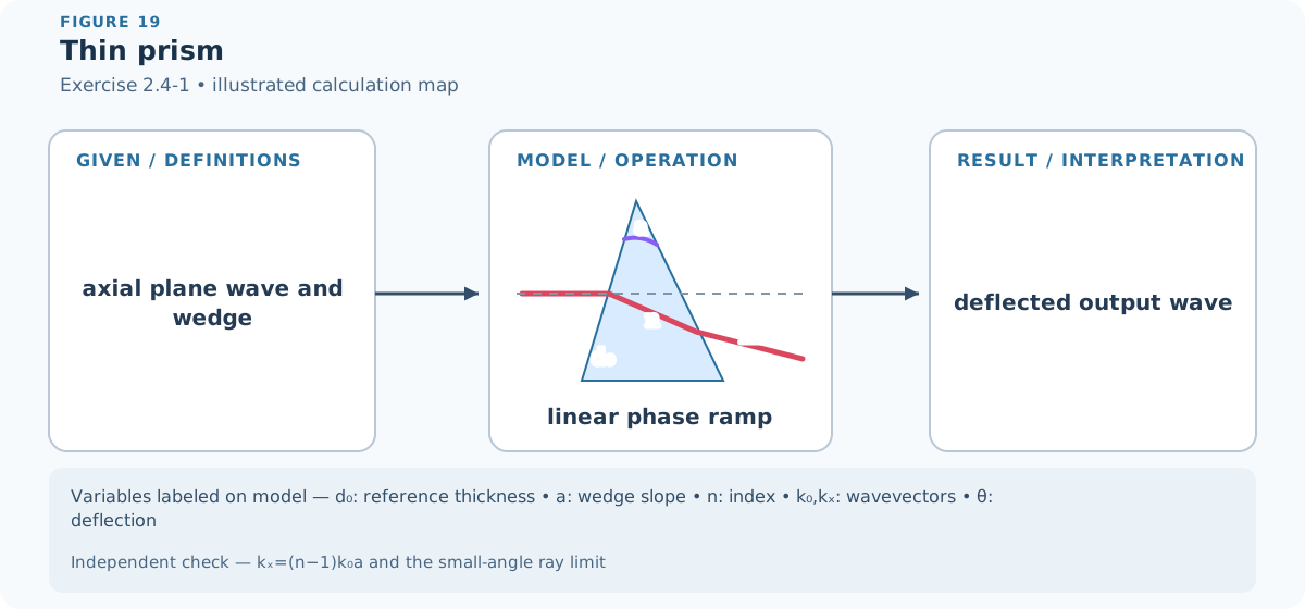
Figure 19 — Exercise 2.4-1: Thin prism. The thickness \(d(x)=\alpha x\) grows toward \(+x\); therefore, with the book’s \(e^{-j\boldsymbol k\cdot\boldsymbol r}\) convention, the output wavevector has \(k_x>0\). The diagram labels the apex angle, thickness, wavevectors, and resulting positive deflection.
Step 2 — Mathematical formulas used. The governing phase law is the variable-thickness-plate transmittance in textbook Eq. (2.4-5), printed p. 53. The result is checked against the thin-prism ray law in textbook Eq. (1.2-7), printed p. 11. The algebra uses phasor identities and small-angle identities.
Step 3 — Worked derivation. At height \(x\), the ray crosses glass of thickness \(d(x)\) and air of thickness \(d_0-d(x)\). Neglecting surface reflection, the two propagation factors multiply:
Factor out the phase accumulated across the reference thickness, \(h_0=e^{-jk_0d_0}\). This gives exactly the form of textbook Eq. (2.4-5):
For the inverted prism, its sloping face gives
so the prism transmittance is a linear phase ramp:
Immediately after the prism, an incident axial plane wave therefore has the form
Because the output propagates in air, \(|\boldsymbol k|=k_0\). If \(\theta\) is measured from \(+z\) toward \(+x\), then
Finally, \(\sin\theta\simeq\theta\) for a thin paraxial prism, so
This is the same magnitude and direction as the ray-optics result in textbook Eq. (1.2-7).
Step 4 — State the numbered result. The principal result obtained in the working is
Step 5 — Check. The phase exponent is dimensionless because \(k_0x\) is dimensionless and \(n-1\) and \(\alpha\) are dimensionless. Setting \(\alpha=0\) or \(n=1\) removes the phase ramp and gives zero deflection. Since \(d(x)\) grows toward \(+x\), the coefficient of \(x\) in the book’s \(e^{-j\boldsymbol k\cdot\boldsymbol r}\) convention gives \(k_x>0\), agreeing with the upward deflection in textbook Fig. 2.4-6. Equation (10) also reproduces the ray result (1.2-7).
Exercise 2.4-2 — Double-convex lens
Brief solution
1. Method. The requested starting point is the variable-thickness plate law, textbook Eq. (2.4-5), printed p. 53:
2. Key step.
Thus the cascade proof gives the same phase and the same focal length as the direct thickness proof.
3. Answer.
Show detailed steps
Step 1 — Definitions and setup. Let \(\rho^2=x^2+y^2\). Put the vertex of the front surface at \(z=0\) and the vertex of the rear surface at \(z=d_0\), where \(d_0\) is the central lens thickness. At radius \(\rho\), the two surface positions are \(z_1(\rho)\) and \(z_2(\rho)\), so the local glass thickness is \(d(\rho)=z_2(\rho)-z_1(\rho)\).
The textbook sign convention gives \(R_1>0\) for the front convex surface and \(R_2<0\) for the rear surface in Fig. 2.4-8. The lens has uniform refractive index \(n\), is surrounded by air, and is thin and paraxial: \(\rho\ll |R_1|,|R_2|\). Surface reflection and absorption are neglected, exactly as in the derivation of textbook Eq. (2.4-5).
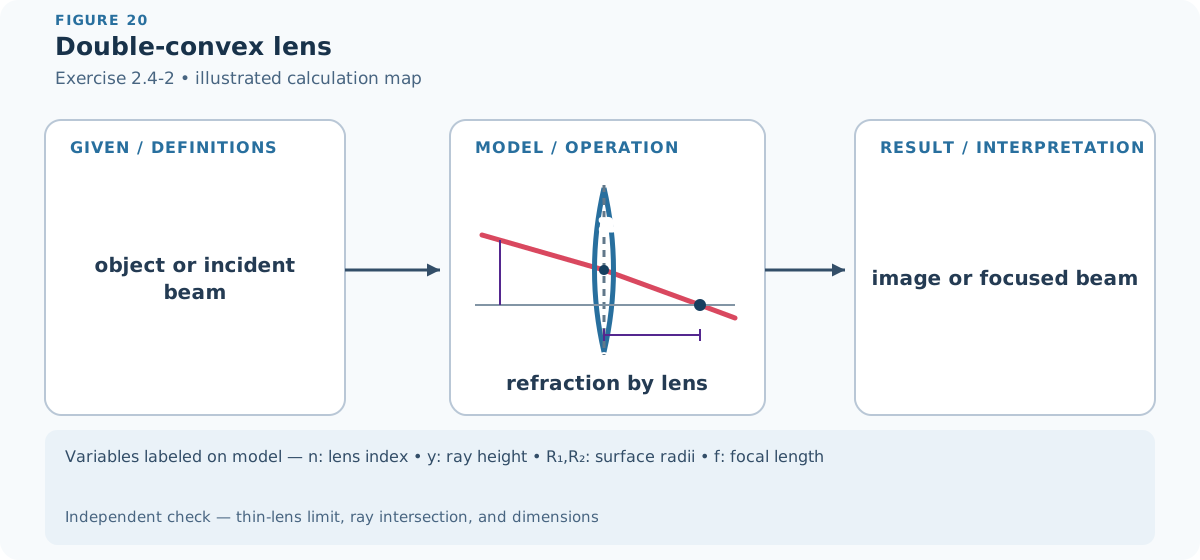
Figure 20 — Exercise 2.4-2: Double-convex lens. The signed surface radii determine the two paraxial sags. Their difference gives the local thickness \(d(\rho)\), whose quadratic part becomes the lens phase.
Step 2 — Mathematical formulas used. The requested starting point is the variable-thickness plate law, textbook Eq. (2.4-5), printed p. 53:
The target is the thin-lens transmittance in textbook Eq. (2.4-9), with the focal length required by Eq. (2.4-11), printed p. 55. The only approximation needed for the geometry is the Taylor expansion \(\sqrt{1-u}\simeq1-u/2\) for \(|u|\ll1\). The algebra also uses phasor identities and small-angle identities.
Step 3 — Worked derivation.
Route A: use the general variable-thickness formula. For either signed spherical radius \(R_i\), the surface sag measured from its vertex is
For \(R_1>0\), this sag is positive, so the front surface moves toward \(+z\) away from its vertex. For \(R_2<0\), it is negative, so the rear surface moves toward \(-z\). Therefore
Subtracting the front position from the rear position gives the glass thickness:
Because \(R_2<0\), the quantity in parentheses is positive. Thus the double-convex lens is thickest on axis and becomes thinner as \(\rho\) increases, as it should.
Insert (14) into the plate law (11):
provided that
This is exactly textbook Eq. (2.4-9) with the focal length of Eq. (2.4-11). The positive sign in the quadratic exponent is required by the book’s \(e^{-j\boldsymbol k\cdot\boldsymbol r}\) convention.
Route B: cascade two plano-convex lenses. Split the lens at an internal plane. The front plano-convex part has power \((n-1)/R_1\). The rear part is reversed; its positive physical curvature magnitude is \(-R_2\), because \(R_2<0\). Hence
Each part contributes a transmittance of the form (2.4-9). Their coordinate-independent phase factors combine into the single constant \(h_0\); multiplying the two transmittances adds their quadratic phases:
Thus the cascade proof gives the same phase and the same focal length as the direct thickness proof.
Step 4 — State the numbered result. The requested complex amplitude transmittance and focal length are
Step 5 — Check.
Symmetric double-convex lens: if \(R_1=R\) and \(R_2=-R\), then \(1/f=2(n-1)/R>0\). Both surfaces add positive converging power; they do not cancel.
Plano-convex limit: letting \(R_2\rightarrow\infty\) gives \(f=R_1/(n-1)\), which is textbook Eq. (2.4-10).
No index contrast: as \(n\rightarrow1\), \(1/f\rightarrow0\) and the transverse quadratic phase disappears.
Dimensions and phase sign: each \(1/R_i\) and \(1/f\) has units of inverse length, while \(k_0\rho^2/f\) is dimensionless. With the textbook phasor convention, the positive quadratic phase in (19) is the converging-lens phase of Eq. (2.4-9).
Exercise 2.4-3 — Lens focusing
Brief solution
1. Method. The working uses exponential, logarithmic, and phasor identities, trigonometric and small-angle identities, and algebraic rearrangement and dimensional checks.
2. Reasoning and answer.
Show detailed steps
Step 1 — Definitions and setup. Symbols are local to this item and follow the chapter convention. Each physical quantity and supplied numerical value is introduced at its first use below; angles are in radians unless a degree symbol is shown, and units are retained through numerical substitution.
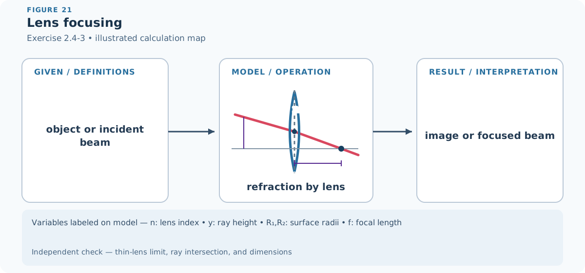
Figure 21 — Exercise 2.4-3: Lens focusing. The diagram identifies the input quantities, physical operation, requested result, variable meanings, and an independent verification route. Every symbol in the variable strip is labeled on the model itself.
Step 2 — Mathematical formulas used. The working uses exponential, logarithmic, and phasor identities, trigonometric and small-angle identities, and algebraic rearrangement and dimensional checks.
Step 3 — Worked derivation. The calculation is kept in symbolic form until the governing relation has been rearranged for the requested quantity.
Detailed step 1. An axial plane wave multiplied by the lens phase becomes \(A_0e^{-jk_0\rho^2/(2f)}\),
Detailed step 2. the converging paraboloidal wave centered at \(z=f\).
Detailed step 3. Incidence angle \(\theta\) contributes \(e^{-jk_0x\theta}\) and translates the focus to \(\boxed{x_f=f\theta}\).
Step 4 — State the numbered result. The principal result obtained in the working is
Step 5 — Check. Equation (20) can be checked by substituting it back into the preceding governing relation and reversing the algebraic steps. The zero-angle or paraxial limit supplies an independent sign and magnitude check whenever that limit is part of the model.
Exercise 2.4-4 — Imaging by phase matching
Brief solution
1. Method. The working uses algebraic rearrangement and dimensional checks.
2. Reasoning and answer.
Show detailed steps
Step 1 — Definitions and setup. Symbols are local to this item and follow the chapter convention. Each physical quantity and supplied numerical value is introduced at its first use below; angles are in radians unless a degree symbol is shown, and units are retained through numerical substitution.
Figure 22 — Exercise 2.4-4: Imaging by phase matching. The diagram identifies the input quantities, physical operation, requested result, variable meanings, and an independent verification route. Every symbol in the variable strip is labeled on the model itself.
Step 2 — Mathematical formulas used. The working uses algebraic rearrangement and dimensional checks.
Step 3 — Worked derivation. The calculation is kept in symbolic form until the governing relation has been rearranged for the requested quantity.
Detailed step 1. The incident paraboloid contributes \(+k\rho^2/(2z_1)\) and the lens \(-k\rho^2/(2f)\).
Detailed step 2. The result equals the outgoing paraboloid phase \(-k\rho^2/(2z_2)\) precisely when \(\boxed{z_1^{-1}+z_2^{-1}=f^{-1}}\).
Step 4 — State the numbered result. The principal result obtained in the working is
Step 5 — Check. Equation (21) can be checked by substituting it back into the preceding governing relation and reversing the algebraic steps. Check that dimensions agree term by term, then test the simplest symmetry or limiting case for the expected sign and scale.
Exercise 2.4-5 — Sinusoidal phase grating
Brief solution
1. Method. The working uses exponential, logarithmic, and phasor identities, trigonometric and small-angle identities, and algebraic rearrangement and dimensional checks.
2. Key step.
Insertion of \(d=d_0[1+\cos(2\pi x/\Lambda)]/2\) gives the stated phase grating. The Jacobi–Anger expansion \(e^{-j\beta\cos Kx}=\sum_q(-j)^qJ_q(\beta)e^{jqKx}\) produces orders
3. Answer.
with complex amplitudes \(h_0(-j)^qJ_q(\beta)\) and \(\beta=(n-1)k_0d_0/2\).
Show detailed steps
Step 1 — Definitions and setup. Symbols are local to this item and follow the chapter convention. Each physical quantity and supplied numerical value is introduced at its first use below; angles are in radians unless a degree symbol is shown, and units are retained through numerical substitution.
Figure 23 — Exercise 2.4-5: Sinusoidal phase grating. The diagram identifies the input quantities, physical operation, requested result, variable meanings, and an independent verification route. Every symbol in the variable strip is labeled on the model itself.
Step 2 — Mathematical formulas used. The working uses exponential, logarithmic, and phasor identities, trigonometric and small-angle identities, and algebraic rearrangement and dimensional checks.
Step 3 — Worked derivation. The calculation is kept in symbolic form until the governing relation has been rearranged for the requested quantity.
Insertion of \(d=d_0[1+\cos(2\pi x/\Lambda)]/2\) gives the stated phase grating. The Jacobi–Anger expansion \(e^{-j\beta\cos Kx}=\sum_q(-j)^qJ_q(\beta)e^{jqKx}\) produces orders
with complex amplitudes \(h_0(-j)^qJ_q(\beta)\) and \(\beta=(n-1)k_0d_0/2\).
Step 4 — Interpret the result. The final relation or conclusion in Step 3 is the requested result. Read its sign, scale, or physical classification using the conventions fixed in Step 1.
Step 5 — Check. Equation (22) can be checked by substituting it back into the preceding governing relation and reversing the algebraic steps. The zero-angle or paraxial limit supplies an independent sign and magnitude check whenever that limit is part of the model.
Exercise 2.4-6 — GRIN plate
Brief solution
1. Method. The working uses algebraic rearrangement and dimensional checks.
2. Key step.
The accumulated phase is \(-k_0n_0d_0+k_0n_0d_0a^2\rho^2/2\); comparison with a thin-lens quadratic phase gives \(\boxed{f=(n_0d_0a^2)^{-1}}\) (the sign follows the propagation convention).
3. Answer.
Show detailed steps
Step 1 — Definitions and setup. Symbols are local to this item and follow the chapter convention. Each physical quantity and supplied numerical value is introduced at its first use below; angles are in radians unless a degree symbol is shown, and units are retained through numerical substitution.
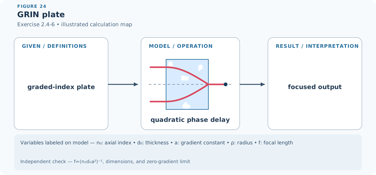
Figure 24 — Exercise 2.4-6: GRIN plate. The diagram identifies the input quantities, physical operation, requested result, variable meanings, and an independent verification route. Every symbol in the variable strip is labeled on the model itself.
Step 2 — Mathematical formulas used. The working uses algebraic rearrangement and dimensional checks.
Step 3 — Worked derivation. The calculation is kept in symbolic form until the governing relation has been rearranged for the requested quantity.
The accumulated phase is \(-k_0n_0d_0+k_0n_0d_0a^2\rho^2/2\); comparison with a thin-lens quadratic phase gives \(\boxed{f=(n_0d_0a^2)^{-1}}\) (the sign follows the propagation convention).
Step 4 — State the numbered result. The principal result obtained in the working is
Step 5 — Check. Equation (23) can be checked by substituting it back into the preceding governing relation and reversing the algebraic steps. Check that dimensions agree term by term, then test the simplest symmetry or limiting case for the expected sign and scale.
Exercise 2.5-1 — Plane/spherical interference
Brief solution
1. Method. The working uses trigonometric and small-angle identities and algebraic rearrangement and dimensional checks.
2. Key step.
Writing the phase difference as \(\phi=k(x^2+y^2)/(2d)+\phi_0\),
3. Answer.
For equal intensities, zeros obey \(k\rho_m^2/(2d)+\phi_0=(2m+1)\pi\); they are concentric circular rings.
Show detailed steps
Step 1 — Definitions and setup. Symbols are local to this item and follow the chapter convention. Each physical quantity and supplied numerical value is introduced at its first use below; angles are in radians unless a degree symbol is shown, and units are retained through numerical substitution.
Figure 25 — Exercise 2.5-1: Plane/spherical interference. The diagram identifies the input quantities, physical operation, requested result, variable meanings, and an independent verification route. Every symbol in the variable strip is labeled on the model itself.
Step 2 — Mathematical formulas used. The working uses trigonometric and small-angle identities and algebraic rearrangement and dimensional checks.
Step 3 — Worked derivation. The calculation is kept in symbolic form until the governing relation has been rearranged for the requested quantity.
Writing the phase difference as \(\phi=k(x^2+y^2)/(2d)+\phi_0\),
For equal intensities, zeros obey \(k\rho_m^2/(2d)+\phi_0=(2m+1)\pi\); they are concentric circular rings.
Step 4 — Interpret the result. The final relation or conclusion in Step 3 is the requested result. Read its sign, scale, or physical classification using the conventions fixed in Step 1.
Step 5 — Check. Equation (24) can be checked by substituting it back into the preceding governing relation and reversing the algebraic steps. The zero-angle or paraxial limit supplies an independent sign and magnitude check whenever that limit is part of the model.
Exercise 2.5-2 — Young interference
Brief solution
1. Method. The working uses trigonometric and small-angle identities and algebraic rearrangement and dimensional checks.
2. Reasoning and answer.
Show detailed steps
Step 1 — Definitions and setup. Symbols are local to this item and follow the chapter convention. Each physical quantity and supplied numerical value is introduced at its first use below; angles are in radians unless a degree symbol is shown, and units are retained through numerical substitution.
Figure 26 — Exercise 2.5-2: Young interference. The diagram identifies the input quantities, physical operation, requested result, variable meanings, and an independent verification route. Every symbol in the variable strip is labeled on the model itself.
Step 2 — Mathematical formulas used. The working uses trigonometric and small-angle identities and algebraic rearrangement and dimensional checks.
Step 3 — Worked derivation. The calculation is kept in symbolic form until the governing relation has been rearranged for the requested quantity.
Detailed step 1. The two Fresnel phases differ by \(2kax/d=kx\theta\),
Detailed step 2. where \(\theta\simeq2a/d\).
Detailed step 3. Thus \(\boxed{I=2I_0[1+\cos(2\pi x\theta/\lambda)]}\) and the fringe spacing is \(\lambda/\theta=\lambda d/(2a)\).
Step 4 — State the numbered result. The principal result obtained in the working is
Step 5 — Check. Equation (25) can be checked by substituting it back into the preceding governing relation and reversing the algebraic steps. The zero-angle or paraxial limit supplies an independent sign and magnitude check whenever that limit is part of the model.
Exercise 2.5-3 — Bragg reflection
Brief solution
1. Method. The working uses trigonometric and small-angle identities and algebraic rearrangement and dimensional checks.
2. Reasoning and answer.
Show detailed steps
Step 1 — Definitions and setup. Symbols are local to this item and follow the chapter convention. Each physical quantity and supplied numerical value is introduced at its first use below; angles are in radians unless a degree symbol is shown, and units are retained through numerical substitution.
Figure 27 — Exercise 2.5-3: Bragg reflection. The diagram identifies the input quantities, physical operation, requested result, variable meanings, and an independent verification route. Every symbol in the variable strip is labeled on the model itself.
Step 2 — Mathematical formulas used. The working uses trigonometric and small-angle identities and algebraic rearrangement and dimensional checks.
Step 3 — Worked derivation. The calculation is kept in symbolic form until the governing relation has been rearranged for the requested quantity.
Detailed step 1. Adjacent planes add path \(2\Lambda\sin\theta\),
Detailed step 2. so \(\phi=2k\Lambda\sin\theta\).
Detailed step 3. The phasors align when \(\boxed{2\Lambda\sin\theta=m\lambda}\); the peak intensity scales as \(M^2\) for \(M\) equal-amplitude planes.
Step 4 — State the numbered result. The principal result obtained in the working is
Step 5 — Check. Equation (26) can be checked by substituting it back into the preceding governing relation and reversing the algebraic steps. The zero-angle or paraxial limit supplies an independent sign and magnitude check whenever that limit is part of the model.
Exercise 2.6-1 — Optical Doppler radar
Brief solution
1. Method. Use the two-frequency interference law, textbook Eq. (2.6-12), together with the moving-delay interference law, textbook Eq. (2.5-6):
2. Key step.
For mirror velocities \(v_m=\pm v\), this is precisely the requested \(f_{\mathrm M}=\pm(2v/c)\nu_0\). An ordinary intensity detector reports the positive oscillation frequency \(|f_{\mathrm M}|\); the sign describes the direction of phase evolution.
3. Answer.
Show detailed steps
Step 1 — Definitions and setup. The textbook uses the similar-looking symbols \(\nu\) for optical frequency and \(v\) for speed. To keep them distinct here, let
\(\nu_0\) be the transmitted optical frequency and \(\lambda_0=c/\nu_0\) its wavelength;
\(v_r\) be the signed line-of-sight target velocity, positive for motion toward the observer and negative for motion away;
\(\Delta\nu\) be the signed Doppler shift, so that the returned frequency is \(\nu_{\mathrm r}=\nu_0+\Delta\nu\);
\(I_{\mathrm{LO}}\) and \(I_{\mathrm r}\) be the intensities of the unshifted local-reference and returned waves at the detector; and
\(\phi_0\) be their constant phase offset at \(t=0\).
The exercise supplies the monostatic (out-and-back) optical Doppler relation
The factor of two occurs because the moving target Doppler-shifts the light on the outward and return parts of the path. This relation assumes \(|v_r|\ll c\) and a target moving along the line of sight.
Figure 28 — Exercise 2.6-1: Optical Doppler radar. The unshifted local oscillator and the return at \(\nu_0+\Delta\nu\) meet at the photodiode. The target’s signed radial velocity determines the electrical beat frequency; its round-trip path gives the factor two.
Step 2 — Mathematical formulas used. Use the two-frequency interference law, textbook Eq. (2.6-12), together with the moving-delay interference law, textbook Eq. (2.5-6):
Here \(d\) is the difference between the distances travelled by the two interferometer waves. The required algebra uses phasor identities, trigonometric identities, and algebraic rearrangement and dimensional checks.
Step 3 — Worked derivation.
Part A: superpose the original and reflected waves. At a fixed point on the detector, write the complex waves in the normalization \(I=|U|^2\):
The detector receives \(U=U_{\mathrm{LO}}+U_{\mathrm r}\). Since a photodetector responds to the time-averaged squared magnitude of the optical field,
where \(\phi_0=\phi_{\mathrm r}-\phi_{\mathrm{LO}}\); changing its sign only changes the arbitrary choice of time origin. The optical-frequency terms near \(\nu_0\) are too fast for the detector electronics, but the cross terms leave an electrical oscillation at the difference frequency. Consequently, the measured beat-frequency magnitude is
If the reference and return have equal intensity \(I_0\), the result reduces to
Part B: turn the result into a radar measurement. Split a narrow-linewidth laser into two paths. Send one path to the target and collect the reflection; retain the other path as a strong local oscillator (LO). Recombine the LO and return on a fast photodiode, then measure \(f_{\mathrm b}\) with an electrical spectrum analyser or frequency counter. Equation (31) gives the magnitude of the radial velocity.
A single real-valued cosine does not reveal the velocity sign because \(\cos(-x)=\cos x\). Direction can be recovered with an in-phase and quadrature detector, which measures the phase rotation direction, or by shifting the LO through a known offset \(f_{\mathrm{off}}\) with an acousto-optic modulator. The Doppler shift then moves the electrical line to one side or the other of the known offset.
Part C: prove the Michelson result from Eq. (2.5-6). Let the moving mirror have axial position \(x(t)=x_0+v_mt\), with signed velocity \(v_m\). Moving that mirror by \(x\) changes its arm’s round-trip path by \(2x\); therefore the path difference in Eq. (2.5-6) is
Substitute this into Eq. (2.5-6):
The signed temporal frequency is the coefficient of \(2\pi t\) inside the cosine. Thus
For mirror velocities \(v_m=\pm v\), this is precisely the requested \(f_{\mathrm M}=\pm(2v/c)\nu_0\). An ordinary intensity detector reports the positive oscillation frequency \(|f_{\mathrm M}|\); the sign describes the direction of phase evolution.
Step 4 — State the numbered result. All three parts requested in the exercise are summarized by
Step 5 — Check.
Stationary target: \(v_r=0\) gives \(\Delta\nu=0\); the interference is constant rather than beating.
Intensity limits: for equal component intensities, the intensity varies between \(0\) and \(4I_0\), matching two-wave interference.
Units: \(\lambda_0f_{\mathrm b}\) has units \(\mathrm{m\,s^{-1}}\), as required for velocity.
Round-trip factor: a mirror displacement of \(\lambda_0/2\) changes the round-trip path by one wavelength and produces one full fringe. A mirror moving at speed \(|v_m|\) therefore produces \(2|v_m|/\lambda_0\) fringes per second.
Direction: replacing \(v_r\) by \(-v_r\) reverses the phase evolution but leaves a single-channel cosine unchanged, explaining why quadrature or an offset reference is needed to measure the sign.
End-of-chapter problems
Problem 2.2-3 — Spherical Helmholtz solution
Brief solution
1. Method. The working uses product, quotient, and chain rules, vector-calculus identities, and exponential, logarithmic, and phasor identities.
2. Reasoning and answer.
Show detailed steps
Definitions and setup. Symbols are local to this item and follow the chapter convention. Each physical quantity and supplied numerical value is introduced at its first use below; angles are in radians unless a degree symbol is shown, and units are retained through numerical substitution.
Mathematical formulas used. The working uses product, quotient, and chain rules, vector-calculus identities, and exponential, logarithmic, and phasor identities.
Worked derivation. The calculation is kept in symbolic form until the governing relation has been rearranged for the requested quantity.
Detailed step 1. For \(U=Ae^{-jkr}/r\),
Detailed step 2. spherical symmetry gives \(\nabla^2U=r^{-2}\partial_r(r^2\partial_rU)=-k^2U\) for \(r>0\); therefore \((\nabla^2+k^2)U=0\) away from the point source.
Numbered result. The principal result obtained in the working is
Check. Equation (37) can be checked by substituting it back into the preceding governing relation and reversing the algebraic steps. Check that dimensions agree term by term, then test the simplest symmetry or limiting case for the expected sign and scale.
Problem 2.2-4 — Spherical-wave intensity
Brief solution
1. Method. The working uses algebraic rearrangement and dimensional checks.
2. Reasoning and answer.
Show detailed steps
Definitions and setup. Symbols are local to this item and follow the chapter convention. Each physical quantity and supplied numerical value is introduced at its first use below; angles are in radians unless a degree symbol is shown, and units are retained through numerical substitution.
Mathematical formulas used. The working uses algebraic rearrangement and dimensional checks.
Worked derivation. The calculation is kept in symbolic form until the governing relation has been rearranged for the requested quantity.
Detailed step 1. Power conservation over a sphere gives \(\boxed{I(r)=P/(4\pi r^2)}\).
Detailed step 2. For \(P=100\ \mathrm W\) at \(r=1\ \mathrm m\), \(\boxed{I=7.96\ \mathrm{W,m^{-2}}}\).
Numbered result. The principal result obtained in the working is
Check. Equation (38) can be checked by substituting it back into the preceding governing relation and reversing the algebraic steps. Check that dimensions agree term by term, then test the simplest symmetry or limiting case for the expected sign and scale. Repeat the substitution with unrounded intermediate values and retain the displayed units; the final unit must have the requested dimension.
Problem 2.2-5 — Cylindrical wave
Brief solution
1. Method. The working uses exponential, logarithmic, and phasor identities and algebraic rearrangement and dimensional checks.
2. Reasoning and answer.
Show detailed steps
Definitions and setup. Symbols are local to this item and follow the chapter convention. Each physical quantity and supplied numerical value is introduced at its first use below; angles are in radians unless a degree symbol is shown, and units are retained through numerical substitution.
Mathematical formulas used. The working uses exponential, logarithmic, and phasor identities and algebraic rearrangement and dimensional checks.
Worked derivation. The calculation is kept in symbolic form until the governing relation has been rearranged for the requested quantity.
Detailed step 1. The outgoing exact solution is \(U=A H_0^{(2)}(k\rho)\) with \(\rho=\sqrt{x^2+z^2}\).
Detailed step 2. For \(k\rho\gg1\), \(U\propto e^{-jk\rho}/\sqrt{\rho}\) and \(\boxed{I=P_\ell/(2\pi\rho)}\),
Detailed step 3. where \(P_\ell\) is power per unit length along the cylinder axis.
Numbered result. The principal result obtained in the working is
Check. Equation (39) can be checked by substituting it back into the preceding governing relation and reversing the algebraic steps. Check that dimensions agree term by term, then test the simplest symmetry or limiting case for the expected sign and scale.
Problem 2.2-6 — Paraxial Helmholtz equation
Brief solution
1. Method. The working uses product, quotient, and chain rules, vector-calculus identities, and exponential, logarithmic, and phasor identities.
2. Reasoning and answer.
Show detailed steps
Definitions and setup. Symbols are local to this item and follow the chapter convention. Each physical quantity and supplied numerical value is introduced at its first use below; angles are in radians unless a degree symbol is shown, and units are retained through numerical substitution.
Mathematical formulas used. The working uses product, quotient, and chain rules, vector-calculus identities, and exponential, logarithmic, and phasor identities.
Worked derivation. The calculation is kept in symbolic form until the governing relation has been rearranged for the requested quantity.
Detailed step 1. Set \(U=Ae^{-jkz}\) in \((\nabla^2+k^2)U=0\).
Detailed step 2. Exact substitution gives \(\nabla_T^2A+\partial_z^2A-2jk\partial_zA=0\); dropping the slowly varying \(\partial_z^2A\) term yields \(\boxed{\nabla_T^2A-2jk\partial_zA=0}\).
Numbered result. The principal result obtained in the working is
Check. Equation (40) can be checked by substituting it back into the preceding governing relation and reversing the algebraic steps. Check that dimensions agree term by term, then test the simplest symmetry or limiting case for the expected sign and scale.
Problem 2.2-7 — Conjugate waves
Brief solution
1. Method. The working uses exponential, logarithmic, and phasor identities and algebraic rearrangement and dimensional checks.
Show detailed steps
Definitions and setup. Symbols are local to this item and follow the chapter convention. Each physical quantity and supplied numerical value is introduced at its first use below; angles are in radians unless a degree symbol is shown, and units are retained through numerical substitution.
Mathematical formulas used. The working uses exponential, logarithmic, and phasor identities and algebraic rearrangement and dimensional checks.
Worked derivation. The calculation is kept in symbolic form until the governing relation has been rearranged for the requested quantity.
Detailed step 1. \(U\) and \(U^*\) have identical intensity but opposite phase and opposite wavefront normals.
Detailed step 2. Thus the conjugate of the stated plane wave travels along \(-(\hat x+\hat y)/\sqrt2\); the conjugate of an outgoing \(e^{-jkr}/r\) spherical wave is an incoming \(e^{+jkr}/r\) wave.
Check. Check that dimensions agree term by term, then test the simplest symmetry or limiting case for the expected sign and scale.
Problem 2.3-1 — Wavefronts in a SELFOC slab
Brief solution
1. Method. The working uses the physical definitions stated in the item; no separate calculus or algebraic identity is required for this qualitative comparison.
Show detailed steps
Definitions and setup. Symbols are local to this item and follow the chapter convention. Each physical quantity and supplied numerical value is introduced at its first use below; angles are in radians unless a degree symbol is shown, and units are retained through numerical substitution.
Mathematical formulas used. The working uses the physical definitions stated in the item; no separate calculus or algebraic identity is required for this qualitative comparison.
Worked derivation. The calculation is kept in symbolic form until the governing relation has been rearranged for the requested quantity.
Detailed step 1. Wavefront normals follow the sinusoidal GRIN rays.
Detailed step 2. Draw curves orthogonal to that ray family: initially planar fronts bend toward the high-index axis,
Detailed step 3. become most curved before the quarter pitch,
Detailed step 4. planar again at a focus crossing,
Detailed step 5. and repeat with the pitch \(2\pi/a\).
Check. For a qualitative conclusion, test every absolute statement against the stated assumptions and at least one limiting case or counterexample.
Problem 2.4-7 — Spherical wave at a plane mirror
Brief solution
1. Method. The working uses trigonometric and small-angle identities.
Show detailed steps
Definitions and setup. No new mathematical symbols are introduced. Technical terms retain their chapter definitions, and each comparison is conditional on the wavelength, material, geometry, and operating assumptions stated below.
Mathematical formulas used. The working uses trigonometric and small-angle identities.
Worked derivation. Evaluate each claim or design choice against the applicable physical definition, then state the assumption that controls the conclusion.
Definitions and setup. No new mathematical symbols are introduced. Technical terms retain their chapter definitions, and each comparison is conditional on the wavelength, material, geometry, and operating assumptions stated below.
Mathematical formulas used. The working uses trigonometric and small-angle identities.
Worked derivation. Evaluate each claim or design choice against the applicable physical definition, then state the assumption that controls the conclusion.
Definitions and setup. No new mathematical symbols are introduced. Technical terms retain their chapter definitions, and each comparison is conditional on the wavelength, material, geometry, and operating assumptions stated below.
Mathematical formulas used. The working uses the physical definitions stated in the item; no separate calculus or algebraic identity is required for this qualitative comparison.
Worked derivation. Evaluate each claim or design choice against the applicable physical definition, then state the assumption that controls the conclusion.
Detailed step 1. Reflect every local plane-wave component by reversing its normal component.
Detailed step 2. Their normals then converge to the mirror image of the source,
Detailed step 3. so the reflected field is a spherical wave centered at the virtual image point,
Detailed step 4. with the mirror reflection coefficient multiplying its amplitude.
Check. For a qualitative conclusion, test every absolute statement against the stated assumptions and at least one limiting case or counterexample.
Check. The zero-angle or paraxial limit supplies an independent sign and magnitude check whenever that limit is part of the model.
Check. The zero-angle or paraxial limit supplies an independent sign and magnitude check whenever that limit is part of the model.
Problem 2.4-8 — Optical path through layers
Brief solution
1. Method. The working uses optical path and Fermat’s principle, exponential, logarithmic, and phasor identities, and algebraic rearrangement and dimensional checks.
2. Reasoning and answer.
Show detailed steps
Definitions and setup. Symbols are local to this item and follow the chapter convention. Each physical quantity and supplied numerical value is introduced at its first use below; angles are in radians unless a degree symbol is shown, and units are retained through numerical substitution.
Mathematical formulas used. The working uses optical path and Fermat’s principle, exponential, logarithmic, and phasor identities, and algebraic rearrangement and dimensional checks.
Worked derivation. The calculation is kept in symbolic form until the governing relation has been rearranged for the requested quantity.
Detailed step 1. Ignoring interface reflections, \(t=\exp[-jk_0\sum_qn_qd_q]\).
Detailed step 2. Equal free-space phase requires \(\boxed{d=\sum_qn_qd_q}\),
Detailed step 3. exactly the optical path length.
Numbered result. The principal result obtained in the working is
Check. Equation (41) can be checked by substituting it back into the preceding governing relation and reversing the algebraic steps. Check that dimensions agree term by term, then test the simplest symmetry or limiting case for the expected sign and scale.
Problem 2.4-9 — Binary phase grating
Brief solution
1. Method. The working uses Fourier-transform and convolution identities, trigonometric and small-angle identities, and algebraic rearrangement and dimensional checks.
2. Reasoning and answer.
Show detailed steps
Definitions and setup. Symbols are local to this item and follow the chapter convention. Each physical quantity and supplied numerical value is introduced at its first use below; angles are in radians unless a degree symbol is shown, and units are retained through numerical substitution.
Mathematical formulas used. The working uses Fourier-transform and convolution identities, trigonometric and small-angle identities, and algebraic rearrangement and dimensional checks.
Worked derivation. The calculation is kept in symbolic form until the governing relation has been rearranged for the requested quantity.
Detailed step 1. For equal half-period levels with transmittances \(t_1,t_2\),
Detailed step 2. Fourier coefficients are \(c_0=(t_1+t_2)/2\) and \(c_q=(t_1-t_2)\sin(q\pi/2)/(q\pi)\) for \(q\ne0\) (up to the chosen cell origin phase).
Detailed step 3. Each coefficient launches an order at \(\boxed{\theta_q\simeq\theta_i+q\lambda/\Lambda}\); even nonzero orders vanish for the symmetric 50% duty cycle.
Numbered result. The principal result obtained in the working is
Check. Equation (42) can be checked by substituting it back into the preceding governing relation and reversing the algebraic steps. Transform dimensions and the expected even/odd or conjugate symmetry provide an independent check on signs and scale factors.
Problem 2.4-10 — Spherical mirror as a phase element
Brief solution
1. Method. The working uses exponential, logarithmic, and phasor identities and algebraic rearrangement and dimensional checks.
2. Reasoning and answer.
Show detailed steps
Definitions and setup. Symbols are local to this item and follow the chapter convention. Each physical quantity and supplied numerical value is introduced at its first use below; angles are in radians unless a degree symbol is shown, and units are retained through numerical substitution.
Mathematical formulas used. The working uses exponential, logarithmic, and phasor identities and algebraic rearrangement and dimensional checks.
Worked derivation. The calculation is kept in symbolic form until the governing relation has been rearranged for the requested quantity.
Detailed step 1. Reflection doubles the surface-sag phase.
Detailed step 2. With \(s\simeq(x^2+y^2)/(2R)\), \(r=h_0e^{-j2k_0s}=h_0e^{-jk_0(x^2+y^2)/R}\).
Detailed step 3. It equals the thin-lens phase for \(\boxed{f=-R/2}\).
Numbered result. The principal result obtained in the working is
Check. Equation (43) can be checked by substituting it back into the preceding governing relation and reversing the algebraic steps. Check that dimensions agree term by term, then test the simplest symmetry or limiting case for the expected sign and scale.
Problem 2.5-4 — Standing wave
Brief solution
1. Method. The working uses trigonometric and small-angle identities and algebraic rearrangement and dimensional checks.
2. Reasoning and answer.
Show detailed steps
Definitions and setup. Symbols are local to this item and follow the chapter convention. Each physical quantity and supplied numerical value is introduced at its first use below; angles are in radians unless a degree symbol is shown, and units are retained through numerical substitution.
Mathematical formulas used. The working uses trigonometric and small-angle identities and algebraic rearrangement and dimensional checks.
Worked derivation. The calculation is kept in symbolic form until the governing relation has been rearranged for the requested quantity.
Detailed step 1. For equal counterpropagating fields, \(U=2A\cos(kz)\) and \(\boxed{I(z)=4I_0\cos^2(kz)}\).
Detailed step 2. Nodes are separated by \(\lambda/2\) and alternate with antinodes.
Numbered result. The principal result obtained in the working is
Check. Equation (44) can be checked by substituting it back into the preceding governing relation and reversing the algebraic steps. The zero-angle or paraxial limit supplies an independent sign and magnitude check whenever that limit is part of the model.
Problem 2.5-5 — Fringe visibility
Brief solution
1. Method. The working uses stationary-value condition, product, quotient, and chain rules, and algebraic rearrangement and dimensional checks.
2. Reasoning and answer.
Show detailed steps
Definitions and setup. Symbols are local to this item and follow the chapter convention. Each physical quantity and supplied numerical value is introduced at its first use below; angles are in radians unless a degree symbol is shown, and units are retained through numerical substitution.
Mathematical formulas used. The working uses stationary-value condition, product, quotient, and chain rules, and algebraic rearrangement and dimensional checks.
Worked derivation. The calculation is kept in symbolic form until the governing relation has been rearranged for the requested quantity.
Detailed step 1. \(I_{max,min}=I_1+I_2\pm2\sqrt{I_1I_2}\),
Detailed step 2. hence \(\boxed{V=2\sqrt{I_1I_2}/(I_1+I_2)}\).
Detailed step 3. Differentiating versus \(I_1/I_2\) gives the maximum \(V=1\) at equal intensities.
Numbered result. The principal result obtained in the working is
Check. Equation (45) can be checked by substituting it back into the preceding governing relation and reversing the algebraic steps. Check that dimensions agree term by term, then test the simplest symmetry or limiting case for the expected sign and scale. Repeat the substitution with unrounded intermediate values and retain the displayed units; the final unit must have the requested dimension.
Problem 2.5-6 — Misaligned Michelson mirror
Brief solution
1. Method. The working uses the physical definitions stated in the item; no separate calculus or algebraic identity is required for this qualitative comparison.
Show detailed steps
Definitions and setup. Symbols are local to this item and follow the chapter convention. Each physical quantity and supplied numerical value is introduced at its first use below; angles are in radians unless a degree symbol is shown, and units are retained through numerical substitution.
Mathematical formulas used. The working uses the physical definitions stated in the item; no separate calculus or algebraic identity is required for this qualitative comparison.
Worked derivation. The calculation is kept in symbolic form until the governing relation has been rearranged for the requested quantity.
Detailed step 1. The returning waves have a linear transverse phase difference and therefore form straight,
Detailed step 2. equally spaced fringes perpendicular to the tilt.
Detailed step 3. Translating the other mirror adds a uniform phase \(4\pi\Delta z/\lambda\),
Detailed step 4. so the whole fringe set slides; one fringe passes a point per \(\lambda/2\) of mirror travel.
Check. For a qualitative conclusion, test every absolute statement against the stated assumptions and at least one limiting case or counterexample.
Problem 2.6-2 — Pulsed spherical wave
Brief solution
1. Method. The working uses Fourier-transform and convolution identities, integration identities, and exponential, logarithmic, and phasor identities.
2. Reasoning and answer.
Show detailed steps
Definitions and setup. Symbols are local to this item and follow the chapter convention. Each physical quantity and supplied numerical value is introduced at its first use below; angles are in radians unless a degree symbol is shown, and units are retained through numerical substitution.
Mathematical formulas used. The working uses Fourier-transform and convolution identities, integration identities, and exponential, logarithmic, and phasor identities.
Worked derivation. The calculation is kept in symbolic form until the governing relation has been rearranged for the requested quantity.
Detailed step 1. Every spectral component propagates as \(e^{-jkr}/r\); inverse Fourier transformation gives \(\boxed{U(r,t)=a(t-r/c)/r}\).
Detailed step 2. For \(\lambda_0=585\ \mathrm{nm}\) and RMS duration \(6\ \mathrm{fs}\),
Detailed step 3. the RMS interval contains \(c\sigma_t/\lambda_0=\boxed{3.08}\) carrier cycles.
Detailed step 4. At \(1\ \mathrm{ps}\) the intensity is a Gaussian spherical shell centered at \(r=ct=0.2998\ \mathrm{mm}\),
Detailed step 5. RMS radial thickness \(c\sigma_t=1.80\ \mathrm{\mu m}\),
Detailed step 6. and amplitude falloff \(1/r^2\).
Numbered result. The principal result obtained in the working is
Check. Equation (46) can be checked by substituting it back into the preceding governing relation and reversing the algebraic steps. Transform dimensions and the expected even/odd or conjugate symmetry provide an independent check on signs and scale factors. Repeat the substitution with unrounded intermediate values and retain the displayed units; the final unit must have the requested dimension.