Chapter 7: Diffraction
Source: Eugene Hecht, Schaum’s Outline of Theory and Problems of Optics (1975), Chapter 7. The entries below cover only the chapter’s Supplementary Problems; prompts are paraphrased and are not reproduced.
Each numbered solution states its assumptions, develops the algebra, substitutes the relevant data, and checks the result. Original SVG illustrations show the ray geometry, field relationships, or calculated curves. Diagrams are schematic unless their axes specify a scale. Source inconsistencies and approximations are identified explicitly rather than silently copied into the answer.
Radiation from a coherent line source
Formula and definitions.
Sum the geometric phasor series \(\sum_{m=0}^{N-1}e^{i2m\alpha}\) and square its magnitude. Principal maxima occur when \(\alpha=q\pi\); zeros occur at the intervening \(N-1\) numerator zeros. A progressive source phase shifts the whole pattern by changing \(\delta_0\).
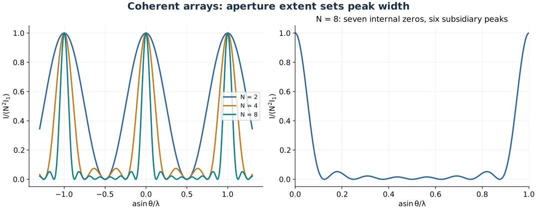
Increasing the coherent element count narrows principal peaks and inserts more subsidiary maxima and zeros.
Problem 7.52 — recover Young’s pattern as a two-element array
Paraphrased task. Recover young’s pattern as a two-element array.
Formula reference. Use (1), its definitions, and the topic illustration.
Worked application.
For equally spaced coherent point emitters, write the phase increment as \(2\alpha=2\pi a\sin\theta/\lambda\). The array factor is \(I_N=I_1[\sin(N\alpha)/\sin\alpha]^2\).
Set \(N=2\) and use \(\sin2\alpha=2\sin\alpha\cos\alpha\). The ratio reduces to \(2\cos\alpha\), including its continuous limit where numerator and denominator both vanish.
Hence \(I_2=4I_1\cos^2(\pi a\sin\theta/\lambda)\), exactly the equal-amplitude Young interference factor. Finite slit width multiplies this by the single-slit envelope.
Result. Young’s two-source pattern is the \(N=2\) array factor.
Check. At broadside the field doubles and the irradiance is four times the one-source value.
Problem 7.53 — count minima and subsidiary maxima between array principals
Paraphrased task. Count minima and subsidiary maxima between array principals.
Formula reference. Use (1), its definitions, and the topic illustration.
Worked application.
Principal maxima occur at \(\alpha=m\pi\), where all \(N\) phasors align and the limiting amplitude is \(N\).
Between \(m\pi\) and \((m+1)\pi\), the numerator vanishes at \(\alpha=m\pi+q\pi/N\), with \(q=1,\ldots,N-1\); the denominator is nonzero there. These are \(N-1\) true minima.
Each interval between consecutive internal zeros contains one subsidiary peak of the uniform-array factor, giving \(N-2\) secondary maxima. The two outer intervals lead into the adjacent principal peaks rather than adding secondary ones.
Result. There are \(N-1\) minima and \(N-2\) secondary maxima between adjacent principal maxima.
Check. For \(N=2\), there is one minimum and no secondary maximum, matching Young interference.
Problem 7.54 — resolve the beam spacing and width of a thirty-two-antenna array
Paraphrased task. Resolve the beam spacing and width of a thirty-two-antenna array.
Formula reference. Use (1), its definitions, and the topic illustration.
Worked application.
The 32-element array has pitch \(a=7\,\mathrm m\) and wavelength \(\lambda=0.21\,\mathrm m\). Principal maxima satisfy \(\sin\theta_m=m\lambda/a\).
Near broadside, adjacent principal maxima are separated by \(\Delta\theta\approx\lambda/a=0.0300\,\mathrm{rad}=1.719^\circ\approx1^\circ43'\).
The first nulls around the central maximum satisfy \(\sin\theta=\pm\lambda/(Na)\). The full null-to-null width is \(2\arcsin[0.21/(32\cdot7)]=0.001875\,\mathrm{rad}=6.45'\).
Result. Principal-lobe separation near broadside \(1.72^\circ\); central null-to-null width \(6.45'\).
Check. The individual 2 m dishes supply a broader element envelope; their diameter is not the array pitch used in the interference factor.
Problem 7.55 — orient the central maximum with progressive source phase
Paraphrased task. Orient the central maximum with progressive source phase.
Formula reference. Use (1), its definitions, and the topic illustration.
Worked application.
Define the phase advance imposed between adjacent emitters as \(\epsilon\), and write the received phase increment as \(\Delta=ka\sin\theta-\epsilon\).
The zeroth-order maximum occurs when adjacent received fields are in phase without an added full turn: \(\Delta=0\).
Therefore \(\theta_0=\arcsin(\epsilon/ka)=\arcsin[\epsilon\lambda/(2\pi a)]\). A propagating zeroth-order direction exists only when the arcsine argument lies between \(-1\) and \(1\).
Result. \(\theta_0=\arcsin[\epsilon\lambda/(2\pi a)]\) with the stated phase-advance convention.
Check. Reversing the definition of which emitter leads changes the steering sign, not its magnitude.
Problem 7.56 — calculate array steering from a thirty-degree phase increment
Paraphrased task. Calculate array steering from a thirty-degree phase increment.
Formula reference. Use (1), its definitions, and the topic illustration.
Worked application.
The frequency \(10^9\,\mathrm{Hz}\) gives \(\lambda=0.30\,\mathrm m\); the pitch is \(a=0.60\,\mathrm m\).
With adjacent phase advance \(\epsilon=30^\circ=\pi/6\), \(\sin\theta_0=(\pi/6)(0.30)/(2\pi\cdot0.60)=1/24\).
Thus \(\theta_0=2.388^\circ\approx2^\circ23'\). The 20-element count narrows the peak but does not change this steering angle, because the required cancellation is between adjacent phases.
Result. The central lobe moves by about \(2.39^\circ\).
Check. The same pitch and frequency give the same steering magnitude as the two-source example in Problem 6.57.
Problem 7.57 — derive specular reflection as an atomic-array maximum
Paraphrased task. Derive specular reflection as an atomic-array maximum.
Formula reference. Use (1), its definitions, and the topic illustration.
Worked application.
Points separated by \(a\) along a smooth reflecting interface are driven by incident phase increment \(\epsilon=ka\sin\theta_i\).
Radiation toward a reflected angle \(\theta\) contributes the opposite geometric increment, so the relative received phase is \(ka(\sin\theta-\sin\theta_i)\).
Constructive addition over the whole interface requires \(\sin\theta=\sin\theta_i\), giving \(\theta=\theta_i\) in the reflected half-space. Atomic spacing is far below the wavelength, so no other propagating grating orders satisfy the condition.
Result. The coherent reradiated principal maximum obeys the law of reflection.
Check. Tangential wave-vector matching is the continuum version of this phased-array argument.
Fraunhofer diffraction by one and two narrow slits
Formula and definitions.
Integrating a uniform slit gives the sinc amplitude. Its zeros set the diffraction envelope, while two-slit interference supplies the faster factor \(\cos^2(\pi a\sin\theta/\lambda)\). Oblique incidence replaces \(\sin\theta\) by the difference from the incident-direction sine.
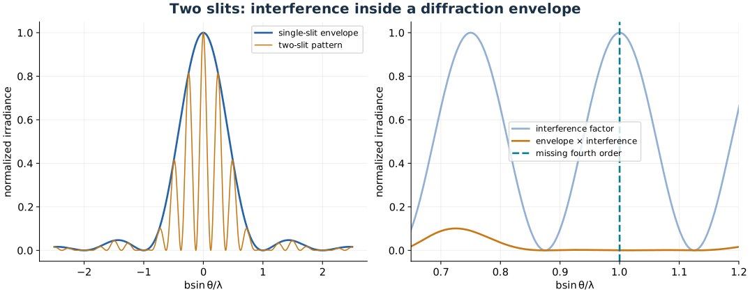
A double-slit interference factor is modulated by its single-slit envelope; missing orders occur at envelope zeros.
Problem 7.58 — prove lens-position independence of focal-plane minima
Paraphrased task. Prove lens-position independence of focal-plane minima.
Formula reference. Use (2), its definitions, and the topic illustration.
Worked application.
A slit minimum is a missing angular component at \(a\sin\theta_m=m\lambda\), independent of any subsequent collecting-lens position.
In the paraxial ray description, a ray arriving at a thin lens with height \(h\) and slope \(u\) exits with slope \(u-h/f\). At the rear focal plane its height is \(h+f(u-h/f)=fu\); the lens intercept height cancels.
Using the geometrical angle-to-screen convention \(z_m=f\tan\theta_m\) gives
\[z_m=\frac{m\lambda f}{\sqrt{a^2-m^2\lambda^2}} \approx\frac{m\lambda f}{a}.\]Translating a sufficiently large collecting lens does not change the angular spectrum; observe its corresponding rear focal plane.
Result. The focal-plane minimum positions depend on \(a,\lambda,f\), not the slit-lens separation.
Check. Clipping by a finite lens or keeping the detector away from the shifted focal plane invalidates the stated invariance.
Problem 7.59 — shift the single-slit pattern for oblique incidence
Paraphrased task. Shift the single-slit pattern for oblique incidence.
Formula reference. Use (2), its definitions, and the topic illustration.
Worked application.
For incidence at \(\theta_i\), the phase gradient across a slit is proportional to \(\sin\theta-\sin\theta_i\), so \(I\propto\operatorname{sinc}^2[\pi a(\sin\theta-\sin\theta_i)/\lambda]\).
The central maximum occurs at \(\theta=\theta_i=30^\circ\). Adjacent minima satisfy \(\sin\theta_m-\sin30^\circ=m\lambda/a\).
Linearize near the maximum: \(\cos30^\circ\,\Delta\theta\approx\lambda/a\). Compared with normal incidence, the local angular spacing increases by \(1/\cos30^\circ=1.1547\).
Result. The pattern shifts to \(30^\circ\) and its local angular fringe scale grows by about \(15.5\%\).
Check. A screen-coordinate width additionally depends on how the screen is oriented relative to the displaced central beam.
Problem 7.60 — overlap minima produced by two wavelengths
Paraphrased task. Overlap minima produced by two wavelengths.
Formula reference. Use (2), its definitions, and the topic illustration.
Worked application.
A single-slit minimum obeys \(a\sin\theta=m\lambda\).
At the common angle, the first minimum for \(\lambda_1\) gives \(a\sin\theta=\lambda_1\), while the third for \(\lambda_2\) gives \(a\sin\theta=3\lambda_2\).
Equate the two right sides; the aperture width and observation geometry cancel.
Result. \(\lambda_1=3\lambda_2\).
Check. The longer wavelength reaches a given angular minimum at a smaller order, consistent with its broader diffraction pattern.
Problem 7.61 — find the half-maximum width of a distant single-slit pattern
Paraphrased task. Find the half-maximum width of a distant single-slit pattern.
Formula reference. Use (2), its definitions, and the topic illustration.
Worked application.
The single-slit profile is \(I/I(0)=(\sin\beta/\beta)^2\), with \(\beta\approx\pi ay/(\lambda L)\).
Half maximum requires \((\sin\beta/\beta)^2=1/2\); the first positive root is \(\beta_{1/2}=1.391557\), not \(\pi/2\).
The full width is
\[W=\frac{2\beta_{1/2}}\pi\frac{\lambda L}{a} =0.885893\frac{(632.8\times10^{-9})(1000)}{10^{-3}} =0.56059\,\mathrm m.\]The printed 632.8 mm corresponds to the rough scale \(\lambda L/a\), not the exact half-irradiance width.
Result. The central-peak FWHM is approximately \(560.6\,\mathrm{mm}\).
Check. The null-to-null width is \(2\lambda L/a=1265.6\,\mathrm{mm}\); it must not be confused with FWHM.
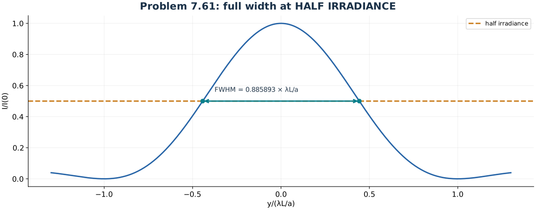
The single-slit half-irradiance crossings give a full width of 0.885893 wavelength times distance divided by slit width.
Problem 7.62 — find first-minimum separation in a lens focal plane
Paraphrased task. Find first-minimum separation in a lens focal plane.
Formula reference. Use (2), its definitions, and the topic illustration.
Worked application.
The first minima satisfy \(\sin\theta_1=\pm\lambda/a\) with \(\lambda=550\,\mathrm{nm}\), \(a=0.25\,\mathrm{mm}\).
Since \(\lambda/a=0.0022\ll1\), use focal-plane positions \(y_{\pm1}\approx\pm f\lambda/a\).
Their separation is \(W=2(0.60)(550\times10^{-9})/(0.25\times10^{-3})=0.00264\,\mathrm m\).
Result. The central null-to-null width is \(2.64\,\mathrm{mm}\).
Check. Each first minimum is only \(1.32\,\mathrm{mm}\) from the centre; the question asks their full separation.
Problem 7.63 — infer focal length from fourth-order minima
Paraphrased task. Infer focal length from fourth-order minima.
Formula reference. Use (2), its definitions, and the topic illustration.
Worked application.
The fourth minima lie at \(y_{\pm4}\approx\pm4\lambda f/a\). Their measured separation is \(\Delta y=8\lambda f/a\).
Isolate the focal length: \(f=a\Delta y/(8\lambda)\).
With \(a=0.25\,\mathrm{mm}\), \(\Delta y=1.25\,\mathrm{mm}\), and \(\lambda=550\,\mathrm{nm}\), \(f=0.071023\,\mathrm m=7.10\,\mathrm{cm}\).
Result. The collecting lens focal length is approximately \(7.1\,\mathrm{cm}\).
Check. The relevant order factor is eight because the measurement spans the negative and positive fourth minima.
Problem 7.64 — count double-slit fringes inside the diffraction envelope
Paraphrased task. Count double-slit fringes inside the diffraction envelope.
Formula reference. Use (2), its definitions, and the topic illustration.
Worked application.
For centre spacing \(a\) and individual slit width \(b\), the central diffraction envelope spans \(-\lambda/b<\sin\theta<\lambda/b\). Interference-order spacing in \(\sin\theta\) is \(\lambda/a\).
Dividing envelope width by fringe spacing gives \((2\lambda/b)/(\lambda/a)=2a/b=2M\). This proves the source’s count of fringe spacings across the envelope.
For an exact count of nominal bright interference orders, require \(|m|<a/b=M\). If \(M\) is an integer, the interior orders are \(m=-(M-1),\ldots,M-1\), giving \(2M-1\); the orders \(\pm M\) are missing at the envelope zeros. The full product’s very weak edge peaks and a visibility threshold can further complicate counting observed bright spots.
Result. \(2M\) is the envelope-width/fringe-spacing ratio; it is not an exact universal count of visible maxima.
Check. An integer order coincident with a single-slit zero cannot be counted as a bright fringe.
Problem 7.65 — infer slit separation from fifteen central bright fringes
Paraphrased task. Infer slit separation from fifteen central bright fringes.
Formula reference. Use (2), its definitions, and the topic illustration.
Worked application.
With \(b=0.25\,\mathrm{mm}\), the approximate width-count rule from Problem 7.64 gives \(15\approx2a/b\), hence \(a\approx1.875\,\mathrm{mm}\).
If instead 15 means the nominal nonmissing interference orders \(0,\pm1,\ldots,\pm7\), their strict condition is \(7<a/b\le8\), or \(1.75<a\le2.00\,\mathrm{mm}\). Merely counting those orders does not uniquely determine \(a\).
If the additional assumption is that the eighth order is exactly missing, \(a/b=8\) and \(a=2.00\,\mathrm{mm}\). The printed 3.75 mm implies \(a/b=15\) and is inconsistent with 15 nominal interior bright orders; the stated seventh-order coincidence is also incompatible with that value.
Result. Width-count estimate: \(a\approx1.875\,\mathrm{mm}\). Exact inference requires an edge-order or fringe-position measurement.
Check. Explicitly distinguish a count of visible peaks, a count of nominal interference orders, and a width divided by a spacing.
Problem 7.66 — infer fringe spacing and slit width from a nine-fringe pattern
Paraphrased task. Infer fringe spacing and slit width from a nine-fringe pattern.
Formula reference. Use (2), its definitions, and the topic illustration.
Worked application.
The printed screen distance is 3 m. With centre spacing \(a=0.4\,\mathrm{mm}\), \(\Delta y\approx\lambda L/a=(550\times10^{-9})(3)/(0.4\times10^{-3})=4.125\,\mathrm{mm}\).
Using the source’s approximate count of nine fringes across the main envelope gives \(9\approx2a/b\); hence \(b\approx2(0.4)/9=0.08889\,\mathrm{mm}\).
This width is an estimate because the weak edge fringes are not assigned a precise detection threshold. Counting exactly nine nominal interference orders would instead constrain \(4<a/b\le5\), or \(0.080\le b<0.100\,\mathrm{mm}\), not uniquely determine the width.
Result. Fringe spacing \(4.125\,\mathrm{mm}\); approximate slit width \(0.089\,\mathrm{mm}\).
Check. The fine fringe spacing determines centre separation, while the much broader envelope determines individual slit width.
Multiple narrow slits and diffraction gratings
Formula and definitions.
The grating equation locates orders; the finite geometric sum sets their width. Applying the Rayleigh criterion to neighboring wavelengths gives \(\mathcal R=mN\). Order overlap requires \(m_1\lambda_1=m_2\lambda_2\).
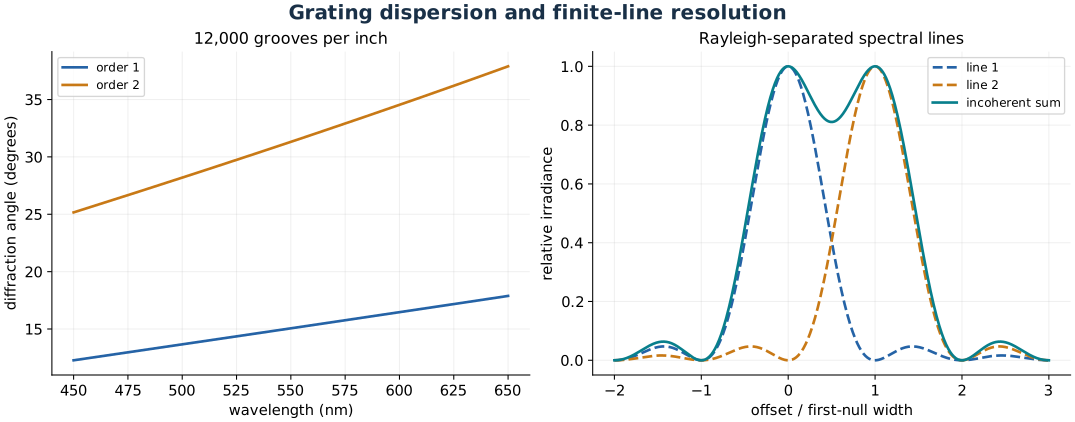
The grating equation separates wavelengths by angle, while finite illuminated line count limits resolution.
Problem 7.67 — recover one- and two-slit limits of the N-slit equation
Paraphrased task. Recover one- and two-slit limits of the n-slit equation.
Formula reference. Use (3), its definitions, and the topic illustration.
Worked application.
Write \(I_N=I_1\operatorname{sinc}^2\beta[\sin(N\alpha)/\sin\alpha]^2\), where \(\beta=\pi b\sin\theta/\lambda\) and \(\alpha=\pi a\sin\theta/\lambda\).
For \(N=1\), the array factor is identically one, leaving the single-slit result \(I_1\operatorname{sinc}^2\beta\).
For \(N=2\), \(\sin2\alpha/\sin\alpha=2\cos\alpha\), giving \(I_2=4I_1\operatorname{sinc}^2\beta\cos^2\alpha\). This separates the individual-slit diffraction envelope from the two-slit interference modulation.
Result. The general grating expression correctly reduces to the one- and two-slit formulas.
Check. At the axis its value is \(N^2I_1\), because fields add coherently.
Problem 7.68 — bound the number of grating principal orders
Paraphrased task. Bound the number of grating principal orders.
Formula reference. Use (3), its definitions, and the topic illustration.
Worked application.
For normal incidence, grating principal orders obey \(a\sin\theta_m=m\lambda\).
A real propagation angle requires \(|\sin\theta_m|\le1\), hence \(|m|\le a/\lambda\) and \(m_{\max}=\lfloor a/\lambda\rfloor\).
At most \(2\lfloor a/\lambda\rfloor+1\) signed orders are geometrically allowed, including zero. Finite slit width can suppress some as missing orders, and an order exactly at grazing is not collected by an ordinary forward screen.
Result. The maximum allowed order magnitude is \(\lfloor a/\lambda\rfloor\) for normal incidence.
Check. Increasing the number of illuminated slits sharpens the allowed orders; it does not create orders beyond the direction-cosine limit.
Problem 7.69 — find the midpoint subsidiary-maximum irradiance for odd N
Paraphrased task. Find the midpoint subsidiary-maximum irradiance for odd n.
Formula reference. Use (3), its definitions, and the topic illustration.
Worked application.
Midway in phase between two principal peaks, \(\alpha=(m+1/2)\pi\), so \(|\sin\alpha|=1\).
For odd \(N\), \(N\alpha\) is also an odd multiple of \(\pi/2\), giving \(|\sin N\alpha|=1\). Thus the squared array factor is one.
Near the central envelope where \(\operatorname{sinc}^2\beta\approx1\), the midpoint irradiance is \(I_1\), while \(I(0)=N^2I_1\). The ratio is \(1/N^2\).
Result. For odd \(N\), the midpoint subsidiary peak has \(I/I(0)\approx1/N^2\).
Check. For even \(N\), the same midpoint has zero numerator and is a minimum, not a subsidiary maximum.
Problem 7.70 — choose focal length for a specified second-order spectrum length
Paraphrased task. Choose focal length for a specified second-order spectrum length.
Formula reference. Use (3), its definitions, and the topic illustration.
Worked application.
The pitch is \(a=25.4\,\mathrm{mm}/12000=2.11667\,\mathrm{\mu m}\). In second order, \(\theta(450\,\mathrm{nm})=\arcsin(0.9/2.11667)=25.163^\circ\) and \(\theta(650\,\mathrm{nm})=37.892^\circ\).
The angular extent is \(\Delta\theta=0.222155\,\mathrm{rad}\). For a collecting lens aimed near the spectrum centre, the local focal-plane approximation \(\Delta y\approx f\Delta\theta\) gives \(f=0.0125/0.222155=0.05627\,\mathrm m\).
This reproduces the source’s \(5.63\,\mathrm{cm}\) angular approximation. Geometry matters at these large absolute angles: a screen perpendicular to the original grating normal with mapping \(y=f\tan\theta\) instead gives \(f=0.0125/(\tan37.892^\circ-\tan25.163^\circ)=4.05\,\mathrm{cm}\).
Result. Approximately \(5.63\,\mathrm{cm}\) for a locally centred collecting-lens angular mapping; specify the optical axis for a nonparaxial screen calculation.
Check. The spectrum spans over \(12^\circ\), so \(f\Delta\theta\) and \(f\Delta(\tan\theta)\) should not be interchanged silently.
Problem 7.71 — prove the upper limit of grating resolving power
Paraphrased task. Prove the upper limit of grating resolving power.
Formula reference. Use (3), its definitions, and the topic illustration.
Worked application.
The ideal Rayleigh resolving power of \(N\) illuminated grating lines in order \(m\) is \(\mathcal R=\lambda/\Delta\lambda=|m|N\).
For normal incidence, the propagating-order condition from Problem 7.68 is \(|m|\le a/\lambda\).
Multiply this inequality by \(N\): \(\mathcal R\le aN/\lambda\). The bound is the illuminated grating width divided by wavelength, up to the usual \(Na\) aperture-width convention.
Result. \(\mathcal R\le aN/\lambda\) for the normal-incidence geometry considered.
Check. The bound changes for oblique incidence; it is not a geometry-independent limit on all grating configurations.
Problem 7.72 — calculate resolving power and wavelength resolution of a grating
Paraphrased task. Calculate resolving power and wavelength resolution of a grating.
Formula reference. Use (3), its definitions, and the topic illustration.
Worked application.
The illuminated number of grooves is \(N=(16000\,\mathrm{in}^{-1})(2.5\,\mathrm{in})=40000\).
Formally, third-order resolving power is \(\mathcal R_3=3N=120000\). In second order \(\mathcal R_2=80000\), giving \(\Delta\lambda_{\min}=550/80000=0.006875\,\mathrm{nm}\).
Check accessibility: the pitch is \(1587.5\,\mathrm{nm}\) and \(3(550)=1650\,\mathrm{nm}>a\). Thus third-order green light is not propagating at normal incidence; the quoted third-order resolving power requires suitable oblique incidence. Second order is accessible normally.
Result. Formal \(\mathcal R_3=120000\); second-order \(\Delta\lambda_{\min}=6.875\times10^{-3}\,\mathrm{nm}\).
Check. A large formal \(mN\) is useful only if the chosen order actually exists in the illumination geometry.
Problem 7.73 — size a grating to resolve adjacent laser longitudinal modes
Paraphrased task. Size a grating to resolve adjacent laser longitudinal modes.
Formula reference. Use (3), its definitions, and the topic illustration.
Worked application.
A mode spacing \(\Delta\nu=150\,\mathrm{MHz}\) at \(\lambda=632.8\,\mathrm{nm}\) demands \(\mathcal R=\nu/\Delta\nu=c/(\lambda\Delta\nu)\approx3.16\times10^6\).
In second order \(N=\mathcal R/2\approx1.58\times10^6\) illuminated grooves.
At \(200\,\mathrm{lines/mm}\), the width is \(W=N/(200\,\mathrm{mm}^{-1})\approx7900\,\mathrm{mm}=7.9\,\mathrm m\). This very large result follows from the given 150 MHz spacing; the printed 79 cm is a factor of ten smaller than these data require.
Result. An ideal second-order grating would need approximately \(7.9\,\mathrm m\) of illuminated width.
Check. The equivalent wavelength separation is only about \(2.0\times10^{-4}\,\mathrm{nm}\), explaining the unusually demanding resolution.
Problem 7.74 — decide which visible diffraction orders can overlap
Paraphrased task. Decide which visible diffraction orders can overlap.
Formula reference. Use (3), its definitions, and the topic illustration.
Worked application.
Different orders overlap when \(m\lambda_m=n\lambda_n\), since they then share the same diffracted angle.
First and second orders require \(\lambda_1=2\lambda_2\). For a conventional 400–700 nm visible interval, even \(2(400)=800\,\mathrm{nm}\) is beyond its red end, so those orders do not overlap. Extending the visible limits can permit a small edge overlap.
Second and third orders require \(\lambda_2=1.5\lambda_3\); for example \(2(600)=3(400)\) nm. They can therefore overlap substantially within the visible band.
Result. First/second overlap is absent or marginal depending on the visible-band definition; second/third overlap is common.
Check. Order-sorting filters remove unwanted wavelengths that share the same grating output angle.
Problem 7.75 — match a third-order wavelength to a fourth-order line
Paraphrased task. Match a third-order wavelength to a fourth-order line.
Formula reference. Use (3), its definitions, and the topic illustration.
Worked application.
At the shared angle, the grating equation gives \(a\sin\theta=3\lambda_3=4\lambda_4\).
Substitute the known fourth-order wavelength \(\lambda_4=490\,\mathrm{nm}\).
Solve \(\lambda_3=(4/3)(490)=653.333\,\mathrm{nm}\).
Result. Third-order \(653.3\,\mathrm{nm}\) overlaps fourth-order \(490\,\mathrm{nm}\).
Check. The lower order must use the longer wavelength to have the same product \(m\lambda\).
Rectangular and circular apertures: Fraunhofer diffraction
Formula and definitions.
Fraunhofer behavior requires the quadratic phase variation across the aperture to be small, giving \(L\gg d^2/\lambda\). A circular aperture produces the Airy pattern; the first zero gives the Rayleigh angular resolution and multiplication by \(f\) gives focal-plane radius.
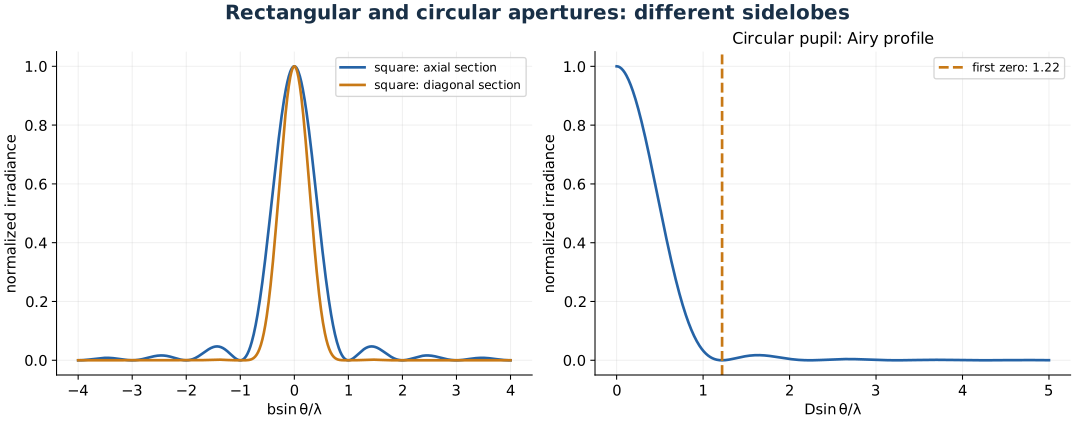
Rectangular pupils give separable sinc patterns; circular pupils give an Airy pattern with its first zero at 1.22 wavelength over diameter.
Problem 7.76 — derive the distance criterion for far-field diffraction
Paraphrased task. Derive the distance criterion for far-field diffraction.
Formula reference. Use (4), its definitions, and the topic illustration.
Worked application.
A spherical wave from an axial point a distance \(L\) away has path \(r(x)=\sqrt{L^2+x^2}\approx L+x^2/(2L)\) across the aperture.
If \(d\) is the maximum transverse coordinate scale, the neglected quadratic phase is at most of order \(\Delta\phi\sim\pi d^2/(\lambda L)\).
Requiring this phase curvature to be small gives \(L\gg d^2/\lambda\), with order-one constants depending on whether \(d\) denotes radius or full width and on the permitted phase error. The same expansion applies to propagation from aperture to screen.
Result. The far-field scale is \(L\gg d^2/\lambda\); \(L>d^2/\lambda\) is only a rough rule of thumb.
Check. For finite source and screen distances, both quadratic contributions must be negligible, or lenses must provide the required wavefront transformation.
Problem 7.77 — estimate direct-view distance behind a circular hole
Paraphrased task. Estimate direct-view distance behind a circular hole.
Formula reference. Use (4), its definitions, and the topic illustration.
Worked application.
The hole radius is 1.25 mm, so its full diameter is \(d=2.5\times10^{-3}\,\mathrm m\).
Apply the source’s full-aperture rule of thumb: \(d^2/\lambda=(2.5\times10^{-3})^2/(632.8\times10^{-9})=9.8767\,\mathrm m\).
A viewing distance greater than roughly 10 m begins the far-field regime on this criterion; use a substantially larger distance for a stricter small-phase-error approximation.
Result. A lens-free Fraunhofer viewing distance is of order \(10\,\mathrm m\) or more.
Check. Using the radius in a formula stated for diameter changes the estimate by a factor of four.
Problem 7.78 — find a diagonal sidelobe of a square aperture
Paraphrased task. Find a diagonal sidelobe of a square aperture.
Formula reference. Use (4), its definitions, and the topic illustration.
Worked application.
A square aperture has \(I/I(0)=\operatorname{sinc}^2\alpha\operatorname{sinc}^2\beta\). Along a diagonal \(\alpha=\beta=u\), so the profile is \((\sin u/u)^4\).
Nonzero side maxima satisfy \(d(\sin u/u)/du=0\), or \(u\cos u-\sin u=0\), equivalently \(\tan u=u\).
For the third side peak, the root between \(3\pi\) and \(7\pi/2\) is \(u=10.90412\). Therefore \(I/I(0)=(\sin u/u)^4=6.956\times10^{-5}\). The simpler midpoint estimate \(u\approx7\pi/2\) gives \(6.84\times10^{-5}\).
Result. The third diagonal side maximum is about \(6.96\times10^{-5}\) of the central irradiance.
Check. Along an axis there is only one sinc-squared factor; along a diagonal two factors suppress the side peaks much more strongly.
Problem 7.79 — scale central irradiance with wavelength and aperture area
Paraphrased task. Scale central irradiance with wavelength and aperture area.
Formula reference. Use (4), its definitions, and the topic illustration.
Worked application.
In scalar Fraunhofer propagation at fixed distance \(L\), the on-axis aperture integral has no transverse phase cancellation: \(U(0)=e^{ikL}U_iA/(i\lambda L)\) for uniform illumination over area \(A\).
Take the squared magnitude: \(I(0)=I_iA^2/(\lambda^2L^2)\).
Thus at fixed incident irradiance and observation distance, the peak scales as \(A^2\) and inversely as \(\lambda^2\). The total transmitted power still scales as \(A\), because a larger aperture also narrows the diffraction pattern.
Result. \(I(0)\propto A^2/\lambda^2\) with illumination and distance held fixed.
Check. Peak irradiance is not total transmitted power; confusing the two would suggest a false energy-conservation problem.
Problem 7.80 — calculate telescope focal-plane Airy radius
Paraphrased task. Calculate telescope focal-plane airy radius.
Formula reference. Use (4), its definitions, and the topic illustration.
Worked application.
A uniformly illuminated circular pupil has first Airy zero at angular radius \(\theta_1\approx1.22\lambda/D\).
At the focal plane its physical radius is \(r_1\approx f\theta_1=1.22\lambda f/D\).
Substitute \(\lambda=550\,\mathrm{nm}\), \(f=1.50\,\mathrm m\), \(D=0.12\,\mathrm m\): \(r_1=8.3875\times10^{-6}\,\mathrm m=0.00839\,\mathrm{mm}\).
Result. The Airy disk radius is approximately \(8.39\,\mathrm{\mu m}\).
Check. The disk diameter is twice this value; the first dark ring defines the boundary used here.
Problem 7.81 — estimate diffraction-limited laser spreading
Paraphrased task. Estimate diffraction-limited laser spreading.
Formula reference. Use (4), its definitions, and the topic illustration.
Worked application.
In the source’s uniform circular-aperture model, the diffraction half-angle to the first zero is \(\theta_1=1.22\lambda/D\).
With \(\lambda=632.8\,\mathrm{nm}\) and initial diameter \(D=2\,\mathrm{mm}\), \(\theta_1=3.8601\times10^{-4}\,\mathrm{rad}\).
At \(L=1000\,\mathrm m\), the first-zero diameter is \(2L\theta_1=0.7720\,\mathrm m\), much larger than the initial 2 mm diameter.
Result. The far-field central-disk diameter is about \(77\,\mathrm{cm}\) under the uniform-aperture model.
Check. A Gaussian laser beam uses a different beam-radius convention and divergence formula; its \(1/e^2\) diameter is not an Airy first-zero diameter.
Problem 7.82 — choose lens diameter for a one-micron image spot
Paraphrased task. Choose lens diameter for a one-micron image spot.
Formula reference. Use (4), its definitions, and the topic illustration.
Worked application.
The requested 1 micrometre spot is a full first-zero diameter, so use \(d_{\rm spot}=2.44\lambda f/D\).
Solve for pupil diameter: \(D=2.44\lambda f/d_{\rm spot}\).
For \(\lambda=450\,\mathrm{nm}\), \(f=225\,\mathrm{mm}\), \(d_{\rm spot}=1\,\mathrm{\mu m}\), the paraxial expression gives \(D=0.24705\,\mathrm m=24.7\,\mathrm{cm}\). This is a fast, high-aperture system, so a real design needs a numerical-aperture/vector-diffraction treatment rather than assuming the paraxial result is exact.
Result. The textbook paraxial aperture estimate is \(D\approx24.7\,\mathrm{cm}\).
Check. The result corresponds to about \(f/0.91\), warning that small-angle pupil geometry is no longer very accurate.
Problem 7.83 — calculate radio-telescope angular resolution
Paraphrased task. Calculate radio-telescope angular resolution.
Formula reference. Use (4), its definitions, and the topic illustration.
Worked application.
For the stated historical telescope, convert \(D=140\,\mathrm{ft}=42.672\,\mathrm m\). The hydrogen-line wavelength is \(\lambda=c/\nu\approx3.0\times10^8/(1.420\times10^9)=0.21127\,\mathrm m\).
The uniform-aperture Rayleigh angle is \(\theta_R=1.22\lambda/D\).
Substitution gives \(\theta_R\approx0.00604\,\mathrm{rad}=0.346^\circ\), close to the rounded \(0.344^\circ\) obtained with \(\lambda=0.21\,\mathrm m\).
Result. Angular resolution is approximately \(6.0\times10^{-3}\,\mathrm{rad}\), or \(0.35^\circ\).
Check. This uses the historical diameter supplied by the exercise, not a claim about present-day telescope rankings.
Problem 7.84 — calculate eye resolution and resolved object spacing
Paraphrased task. Calculate eye resolution and resolved object spacing.
Formula reference. Use (4), its definitions, and the topic illustration.
Worked application.
The diffraction-limited angular separation in object space is \(\Delta\phi=1.22\lambda_0/D\) for the air-side pupil.
With \(\lambda_0=550\,\mathrm{nm}\) and \(D=2.5\,\mathrm{mm}\), \(\Delta\phi=2.684\times10^{-4}\,\mathrm{rad}\).
At \(L=1000\,\mathrm m\), the minimum transverse source spacing is \(s\approx L\Delta\phi=0.2684\,\mathrm m=26.84\,\mathrm{cm}\). Internal ocular refraction changes the retinal angle, not this external source separation calculation.
Result. Ideal angular resolution \(2.68\times10^{-4}\,\mathrm{rad}\); source separation at 1 km \(26.8\,\mathrm{cm}\).
Check. Real visual acuity also depends on aberrations, contrast, retinal sampling, and illumination; this is only the diffraction limit.
Problem 7.85 — find headlight resolution distance for a dark-adapted pupil
Paraphrased task. Find headlight resolution distance for a dark-adapted pupil.
Formula reference. Use (4), its definitions, and the topic illustration.
Worked application.
Convert the headlight spacing: \(s=43\,\mathrm{in}=1.0922\,\mathrm m\).
A 4 mm pupil at 550 nm has Rayleigh angle \(\theta_R=1.22(550\times10^{-9})/0.004=1.6775\times10^{-4}\,\mathrm{rad}\).
Set the apparent separation \(s/L\) equal to \(\theta_R\): \(L=s/\theta_R=6511\,\mathrm m\approx6.51\,\mathrm{km}\).
Result. The ideal diffraction-limited just-resolvable distance is about \(6.5\,\mathrm{km}\).
Check. This ignores atmospheric blur and glare; it is not a practical guaranteed nighttime viewing distance.
Fresnel diffraction: circular systems
Formula and definitions.
Successive Fresnel-zone boundaries differ in optical path by \(\lambda/2\), so adjacent zone amplitudes nearly cancel. Convert every open annulus to the difference of two cumulative vibration-curve vectors and sum complex amplitudes before squaring. A zone plate passes alternate zones, making their surviving contributions add near a focus.
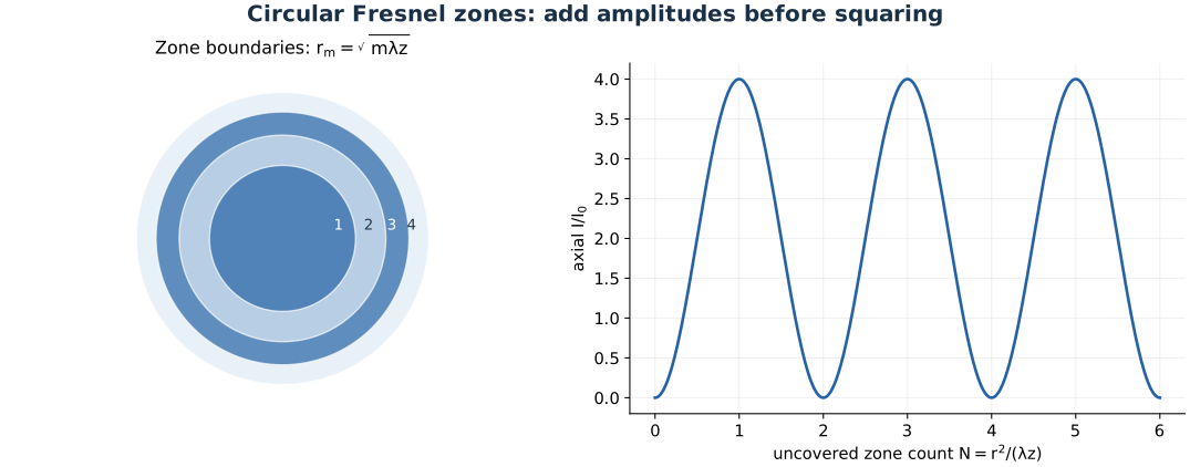
Circular-aperture axial irradiance oscillates with the exposed Fresnel-zone count rather than increasing monotonically with radius.
Problem 7.86 — count Fresnel zones uncovered by a circular aperture
Paraphrased task. Count fresnel zones uncovered by a circular aperture.
Formula reference. Use (5), its definitions, and the topic illustration.
Worked application.
For normally incident plane waves observed on axis at distance \(z\), a radius \(r\) adds path \(\Delta\approx r^2/(2z)\).
A half-period Fresnel zone corresponds to \(\Delta=m\lambda/2\), so \(r_m^2=m\lambda z\) and the exposed zone count is \(N=r^2/(\lambda z)\).
The hole radius is \(r=0.005\,\mathrm m\), not 0.01 m. Hence \(N=0.005^2/[(500\times10^{-9})(0.5)]=100\).
Result. The aperture uncovers approximately 100 Fresnel half-period zones.
Check. The Fresnel-zone count uses radius squared; inserting the diameter would overestimate the count by four.
Problem 7.87 — find aperture radii giving on-axis maxima and minima
Paraphrased task. Find aperture radii giving on-axis maxima and minima.
Formula reference. Use (5), its definitions, and the topic illustration.
Worked application.
For a circular aperture, normalized axial field in the Fresnel approximation is \(U/U_0=1-e^{i\pi N}\), where \(N=r^2/(\lambda z)\).
Thus \(I/I_0=4\sin^2(\pi N/2)\): odd zone counts give maxima and even counts give minima.
With \(\lambda z=(500\times10^{-9})(2.25)=1.125\times10^{-6}\,\mathrm{m^2}\), the first three odd-zone radii are \(\sqrt{1,3,5}\sqrt{\lambda z}=1.061,1.837,2.372\,\mathrm{mm}\). The first three nonzero even-zone radii are \(1.500,2.121,2.598\,\mathrm{mm}\).
Result. Maxima at \(1.06,1.84,2.37\,\mathrm{mm}\); minima at \(1.50,2.12,2.60\,\mathrm{mm}\), continuing by \(r_m=\sqrt{m\lambda z}\).
Check. Adding more aperture area can reduce on-axis irradiance because adjacent zones arrive approximately out of phase.
Problem 7.88 — find axial irradiance behind a helium-neon aperture
Paraphrased task. Find axial irradiance behind a helium-neon aperture.
Formula reference. Use (5), its definitions, and the topic illustration.
Worked application.
Calculate the exposed zone count: \(N=(0.7955\times10^{-3})^2/[(632.8\times10^{-9})(2)]\approx0.50002\).
The normalized axial field is \(1-e^{i\pi N}\). For exactly half a zone this is \(1-i\), whose squared magnitude is 2.
Equivalently \(I/I_0=4\sin^2(\pi N/2)\approx4\sin^2(\pi/4)=2\).
Result. The axial irradiance is approximately \(2I_0\).
Check. Half a Fresnel zone does not mean half the unobstructed irradiance; amplitudes and their relative phase determine the result.
Problem 7.89 — sum annular-zone contributions for a shaped aperture
Paraphrased task. Sum annular-zone contributions for a shaped aperture.
Formula reference. Use (5), its definitions, and the topic illustration.
Worked application.
At \(\lambda=500\,\mathrm{nm}\), \(z=4\,\mathrm m\), the first two zone radii are \(r_1=\sqrt{\lambda z}=1.414\,\mathrm{mm}\) and \(r_2=\sqrt{2\lambda z}=2.000\,\mathrm{mm}\).
The illustrated aperture transmits the full first zone plus a \(90^\circ\) sector, one quarter, of the second zone. A full first zone contributes \(2U_0\), while the full second contributes \(-2U_0\) in the equal-zone approximation.
Since phase on axis is independent of azimuth, the sector contributes its angular fraction of the field: \(U/U_0=2-(1/4)2=3/2\). Therefore \(I=(3/2)^2(40)=90\,\mathrm{W\,m^{-2}}\).
Result. The axial irradiance is \(90\,\mathrm{W\,m^{-2}}\) in the Fresnel-zone approximation.
Check. Use a quarter of the second-zone amplitude, not a quarter of its irradiance; the sectors interfere coherently.
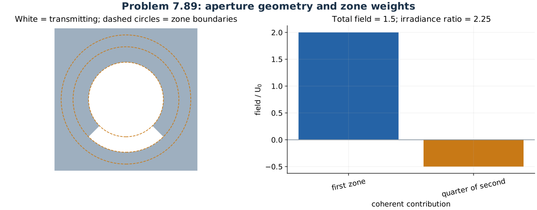
Zone-sector aperture for Problem 7.89: the whole first zone and one quarter of the second zone are open.
Problem 7.90 — use the vibration curve for one-and-a-half open zones
Paraphrased task. Use the vibration curve for one-and-a-half open zones.
Formula reference. Use (5), its definitions, and the topic illustration.
Worked application.
One and a half uncovered zones means \(N=1.5\), or an aperture-edge phase \(\pi N=3\pi/2\).
The circular-aperture field is \(U/U_0=1-e^{i3\pi/2}=1+i\).
Squaring gives \(I/I_0=|1+i|^2=2\). The same value follows from \(4\sin^2(3\pi/4)\).
Result. \(I=2I_0\).
Check. The half-zone and one-and-a-half-zone apertures have different field phases but equal axial irradiances.
Problem 7.91 — find axial irradiance through a second shaped aperture
Paraphrased task. Find axial irradiance through a second shaped aperture.
Formula reference. Use (5), its definitions, and the topic illustration.
Worked application.
At \(\lambda z=2\times10^{-6}\,\mathrm{m^2}\), the source figure’s upper semicircle of radius 1.414 mm ends at zone 1; its lower semicircle of radius 2.449 mm ends at zone 3.
Any full odd-zone circular aperture contributes \(2U_0\) on axis in this approximation. Each semicircle contributes half of its respective full aperture field, so the two contributions are \(U_0\) and \(U_0\).
Add before squaring: \(U=2U_0\), hence \(I=4I_0=4(25)=100\,\mathrm{W\,m^{-2}}\).
Result. The on-axis irradiance is \(100\,\mathrm{W\,m^{-2}}\).
Check. Although the semicircle areas differ, each includes an odd number of half-period zones and gives the same normalized axial field.
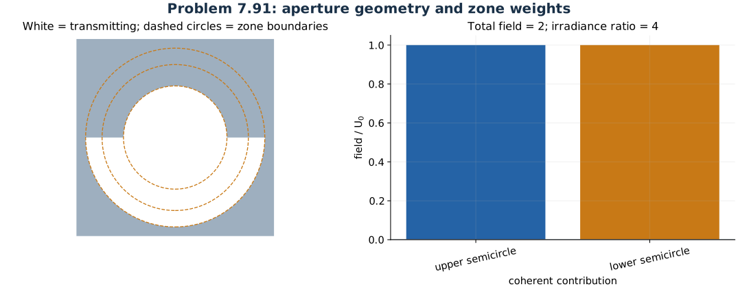
Two semicircular openings end at the first and third Fresnel-zone boundaries; their on-axis amplitudes reinforce.
Problem 7.92 — evaluate an annular obstruction with the vibration curve
Paraphrased task. Evaluate an annular obstruction with the vibration curve.
Formula reference. Use (5), its definitions, and the topic illustration.
Worked application.
The opaque shape blocks the first full zone and two opposite \(90^\circ\) sectors of the second zone, with radii \(r_1=1.414\,\mathrm{mm}\), \(r_2=2\,\mathrm{mm}\) at the stated wavelength and distance.
The field that would pass through the complementary shaped aperture is \(U_{\rm blocked}=2U_0+\tfrac12(-2U_0)=U_0\).
Apply Babinet’s principle to complex fields: \(U_{\rm obstruction}=U_0-U_{\rm blocked}=0\). Equivalently, the first-zone disk alone leaves \(-U_0\); blocking half the next zone adds \(+U_0\) and cancels it.
Result. The axial irradiance is approximately zero.
Check. Babinet subtracts complex amplitudes, not intensities. Rounded zone radii and nonparaxial corrections prevent a perfectly exact physical zero.
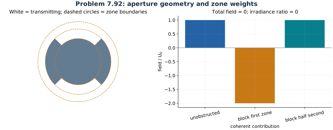
The blocked first zone plus half the second zone has the same axial field as the unobstructed beam; their difference is nearly zero.
Problem 7.93 — derive zone-plate focal length and first-zone radius
Paraphrased task. Derive zone-plate focal length and first-zone radius.
Formula reference. Use (5), its definitions, and the topic illustration.
Worked application.
For source and image distances \(p,q\), the extra path through radius \(r\) is \(\Delta\approx r^2/(2p)+r^2/(2q)\).
At the \(m`th zone boundary, set :math:\)Delta=mlambda/2`. Then \(r_m^2(1/p+1/q)=m\lambda\), or \(1/p+1/q=1/f\) with \(f=r_m^2/(m\lambda)\).
With \(p=q=5\,\mathrm m\), \(f=2.5\,\mathrm m\). The first-zone radius is \(r_1=\sqrt{\lambda f}=\sqrt{(500\times10^{-9})(2.5)}=1.118\,\mathrm{mm}=0.1118\,\mathrm{cm}\).
Result. The zone-plate focal length is \(r_m^2/(m\lambda)\); the first radius here is \(1.12\,\mathrm{mm}\).
Check. The focal length varies inversely with wavelength, so a zone plate is strongly chromatic.
Problem 7.94 — calculate zone-plate focus irradiance with only the first zone open
Paraphrased task. Calculate zone-plate focus irradiance with only the first zone open.
Formula reference. Use (5), its definitions, and the topic illustration.
Worked application.
The unobstructed on-axis wave is the coherent sum of all half-period zones; their alternating contributions leave approximately half the first-zone field.
Equivalently, the Fresnel aperture formula at \(N=1\) gives \(U/U_0=1-e^{i\pi}=2\).
With all other zones blocked, the irradiance is therefore \(I/I_0=|2|^2=4\).
Result. The single first-zone opening produces approximately \(4I_0\) at the focus.
Check. This local concentration does not increase total transmitted power; other observation points receive less light.
Problem 7.95 — find zone-plate focal and image distances
Paraphrased task. Find zone-plate focal and image distances.
Formula reference. Use (5), its definitions, and the topic illustration.
Worked application.
Use \(m=8\), \(r_8=4.5\,\mathrm{mm}\), and \(\lambda=650\,\mathrm{nm}\) in \(f=r_8^2/(m\lambda)\).
This gives \(f=(4.5\times10^{-3})^2/[8(650\times10^{-9})]=3.89423\,\mathrm m\).
For \(p=7.788\,\mathrm m\), \(q=(1/f-1/p)^{-1}\approx7.789\,\mathrm m\). Since \(p\) is essentially \(2f\), the image distance is essentially \(2f\) as well.
Result. \(f\approx3.894\,\mathrm m\); image distance approximately \(7.79\,\mathrm m\).
Check. Use the zone-boundary index 8, not the count of transparent rings, when applying \(r_m^2=m\lambda f\).
Fresnel diffraction: straight edges
Formula and definitions.
Map each physical edge to its dimensionless Fresnel coordinate \(u\). The Cornu-spiral chord between the two edge points is the complex field; its squared length, with the unobstructed normalization, is irradiance. For complementary apertures, Babinet’s principle adds fields—not irradiances—to the unobstructed field.
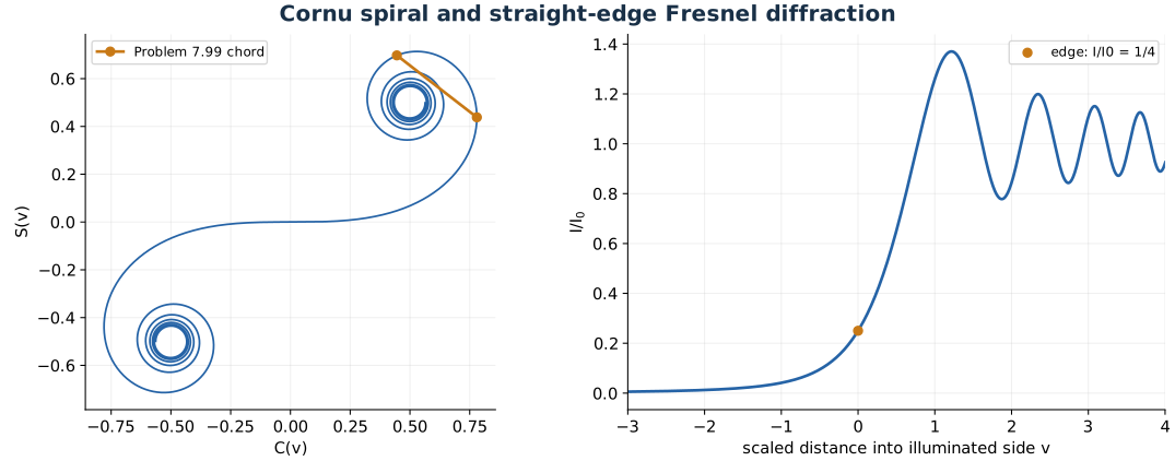
The complex field is a chord of the Cornu spiral. A straight edge gives one quarter of unobstructed irradiance at the shadow boundary.
Problem 7.96 — prove that a very wide slit approaches unobstructed irradiance
Paraphrased task. Prove that a very wide slit approaches unobstructed irradiance.
Formula reference. Use (6), its definitions, and the topic illustration.
Worked application.
Let \(F(v)=C(v)+iS(v)=\int_0^v e^{i\pi u^2/2}\,du\). For a centred slit with scaled half-width \(v\), its normalized irradiance is \(I/I_0=\tfrac12|F(v)-F(-v)|^2\).
Both Fresnel integrals are odd, so this becomes \(I/I_0=2[C(v)^2+S(v)^2]\).
A very wide slit has \(v\to\infty\), where \(C,S\to1/2\). Thus \(I/I_0\to2[(1/2)^2+(1/2)^2]=1\).
Result. The axial irradiance approaches the unobstructed value \(I_0\) as slit width increases without bound.
Check. The approach is oscillatory because successive admitted strips add at changing phases; it is not monotonic.
Problem 7.97 — derive Cornu-spiral slope and locate horizontal and vertical tangencies
Paraphrased task. Derive cornu-spiral slope and locate horizontal and vertical tangencies.
Formula reference. Use (6), its definitions, and the topic illustration.
Worked application.
Parameterize the Cornu spiral by \((C(v),S(v))\). Differentiation gives \(C'(v)=\cos(\pi v^2/2)\) and \(S'(v)=\sin(\pi v^2/2)\).
Therefore \(dS/dC=\tan(\pi v^2/2)\). The directed tangent angle is \(\beta=\pi v^2/2\) modulo \(2\pi\); also \(\sqrt{C'^2+S'^2}=1\), so \(v\) is signed arc length.
Horizontal tangents require \(v^2=2m\), while vertical tangents require \(v^2=2m+1\). Include both signs of \(v\); the origin itself is also a horizontal tangent.
Result. Horizontal tangents: \(v=0,\pm\sqrt2,\pm\sqrt4,\ldots\); vertical tangents: \(v=\pm1,\pm\sqrt3,\ldots\).
Check. The tangent slope repeats modulo \(\pi\), but the directed tangent retains the sign information of both derivatives.
Problem 7.98 — evaluate a line-source central slit irradiance and Cornu arc
Paraphrased task. Evaluate a line-source central slit irradiance and cornu arc.
Formula reference. Use (6), its definitions, and the topic illustration.
Worked application.
For finite source and screen distances \(p=2\,\mathrm m\), \(q=3\,\mathrm m\), the reduced distance is \(L_{\rm eff}=pq/(p+q)=1.2\,\mathrm m\).
A centred slit of width \(b=0.25\,\mathrm{mm}\) has scaled endpoints \(v_\pm=\pm(b/2)\sqrt{2/(\lambda L_{\rm eff})}=\pm0.208333\). The Cornu arc length is \(\Delta v=0.416667\).
At the positive endpoint, \(C=0.208237\), \(S=0.004733\). Thus \(I/I_0=2(C^2+S^2)=0.08677\), approximately the source’s 0.09.
Result. Axial irradiance \(0.0868I_0\); Cornu arc length \(0.417\).
Check. The normalization \(I_0\) is the unobstructed irradiance at the observation point, not necessarily the irradiance at the slit.
Problem 7.99 — evaluate an off-axis slit irradiance under plane-wave illumination
Paraphrased task. Evaluate an off-axis slit irradiance under plane-wave illumination.
Formula reference. Use (6), its definitions, and the topic illustration.
Worked application.
For plane-wave illumination the scale is \(v=(x-y)\sqrt{2/(\lambda z)}\). Here \(\sqrt{2/(640\times10^{-9}\cdot2)}=1250\,\mathrm{m}^{-1}\).
With slit edges \(x=\pm0.2\,\mathrm{mm}\) and observation point \(y=-1\,\mathrm{mm}\), the endpoints are \(v_1=1.0\), \(v_2=1.5\).
The Fresnel integrals give \(\Delta C=0.445261-0.779893=-0.334632\) and \(\Delta S=0.697505-0.438259=0.259246\). Therefore \(I/I_0=(\Delta C^2+\Delta S^2)/2=0.089594\).
Result. The irradiance 1 mm below the axis is \(0.0896I_0\).
Check. A symmetric slit gives the same irradiance 1 mm above the axis, although the signed Fresnel endpoints differ.
Problem 7.100 — maximize on-axis irradiance of a variable-width slit
Paraphrased task. Maximize on-axis irradiance of a variable-width slit.
Formula reference. Use (6), its definitions, and the topic illustration.
Worked application.
For a centred slit with scaled half-width \(v\), \(I/I_0=2[C(v)^2+S(v)^2]\).
Differentiate with respect to width parameter:
\[\frac{d(I/I_0)}{dv} =4\left[C(v)\cos\frac{\pi v^2}{2} +S(v)\sin\frac{\pi v^2}{2}\right].\]The first and largest positive maximum occurs at \(v\approx1.20938\), where this derivative changes from positive to negative. Evaluation gives \(I_{\max}/I_0\approx1.80142\); later oscillations tend toward one.
Result. The greatest axial irradiance is approximately \(1.80I_0\).
Check. On the Cornu diagram this is the longest chord joining the symmetric points \(F(-v)\) and \(F(v)\).
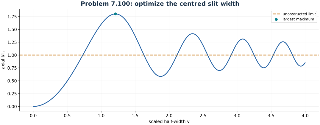
The largest axial slit irradiance occurs at scaled half-width 1.20938; subsequent width oscillations tend toward the unobstructed value.
Problem 7.101 — explain the narrow-slit approach to Fraunhofer behavior
Paraphrased task. Explain the narrow-slit approach to fraunhofer behavior.
Formula reference. Use (6), its definitions, and the topic illustration.
Worked application.
Write the slit field as \(U(y)\propto\int_{-b/2}^{b/2}\exp[i\pi(x-y)^2/(\lambda z)]\,dx\) for plane-wave incidence.
Expand the square: the phase contains a constant \(\pi y^2/(\lambda z)\), a linear term \(-2\pi xy/(\lambda z)\), and a quadratic term \(\pi x^2/(\lambda z)\). If \(b^2/(\lambda z)\ll1\), neglect the last term across the slit.
The remaining integral is \(b\operatorname{sinc}[\pi by/(\lambda z)]\) times an irrelevant overall phase. On the Cornu spiral, the short integration arc has almost linear phase variation across the slit, and its chord develops the familiar far-field near-cancellations.
Result. A narrow enough slit approaches the Fraunhofer sinc-squared pattern when its quadratic aperture phase is negligible.
Check. A small aperture alone is not the criterion: its width must be small compared with the Fresnel scale \(\sqrt{\lambda z}\).
Problem 7.102 — choose a slit width that maximizes axial irradiance
Paraphrased task. Choose a slit width that maximizes axial irradiance.
Formula reference. Use (6), its definitions, and the topic illustration.
Worked application.
Interpret the source’s wavelength typo as \(500\,\mathrm{nm}\), appropriate to the optical context. With \(p=1\,\mathrm m\), \(q=4\,\mathrm m\), \(L_{\rm eff}=pq/(p+q)=0.8\,\mathrm m\).
The greatest axial slit maximum from Problem 7.100 has scaled endpoints \(\pm1.20938\), hence \(\Delta v=2.41875\).
Convert arc length to physical width: \(b=\Delta v\sqrt{\lambda L_{\rm eff}/2}=2.41875\sqrt{(500\times10^{-9})(0.8)/2}=1.0817\,\mathrm{mm}\). A coarse graphical Cornu reading gives a value near the source’s 1.13 mm, but numerical maximization gives 1.08 mm.
Result. The numerically optimized slit width is approximately \(1.08\,\mathrm{mm}\) for the first, largest axial maximum.
Check. Other wider local maxima exist; stating the first/largest maximum makes the width selection unambiguous.
Problem 7.103 — prove the quarter-irradiance value opposite a half-plane edge
Paraphrased task. Prove the quarter-irradiance value opposite a half-plane edge.
Formula reference. Use (6), its definitions, and the topic illustration.
Worked application.
Opposite a straight edge, exactly one half of the unobstructed integration plane is open. In the one-dimensional Fresnel integral the aperture runs from \(v=0\) to \(+\infty\).
Its complex Cornu displacement is \(F(\infty)-F(0)=(1+i)/2\), half the full-plane displacement \(F(\infty)-F(-\infty)=1+i\).
The field is therefore \(U=U_0/2\), and its irradiance is \(I=|U/U_0|^2I_0=I_0/4\).
Result. At the geometrical shadow boundary, \(I=I_0/4\).
Check. Half the coherent field gives one quarter of the irradiance, not one half.
Problem 7.104 — locate the first maximum and minimum behind a straight edge
Paraphrased task. Locate the first maximum and minimum behind a straight edge.
Formula reference. Use (6), its definitions, and the topic illustration.
Worked application.
Let \(y>0\) point into the illuminated region and define \(v=y\sqrt{2/(\lambda z)}\). The edge profile is \(I/I_0=\tfrac12[(1/2+C(v))^2+(1/2+S(v))^2]\).
Set its derivative to zero: \((1/2+C)\cos(\pi v^2/2)+(1/2+S)\sin(\pi v^2/2)=0\). The first maximum is at \(v=1.21720\); the next, first minimum, is at \(v=1.87252\).
With \(\lambda=400\,\mathrm{nm}\), \(z=10\,\mathrm m\), the conversion scale is \(\sqrt{\lambda z/2}=1.41421\,\mathrm{mm}\). Thus \(y_{\max}=1.721\,\mathrm{mm}\) and \(y_{\min}=2.648\,\mathrm{mm}\). These refine the source’s graphical estimates.
Result. First maximum \(1.72\,\mathrm{mm}\) into the lit side; first minimum \(2.65\,\mathrm{mm}\) into the lit side.
Check. There is no mirrored sequence of equal-brightness fringes deep in the shadow; the straight-edge pattern is asymmetric.
Problem 7.105 — find and sketch the central irradiance behind a narrow opaque strip
Paraphrased task. Find and sketch the central irradiance behind a narrow opaque strip.
Formula reference. Use (6), its definitions, and the topic illustration.
Worked application.
For strip width \(b=1.766\,\mathrm{mm}\), \(\lambda=693.4\,\mathrm{nm}\), \(z=1\,\mathrm m\), the centred complementary slit has \(v_\pm=\pm(b/2)\sqrt{2/(\lambda z)}=\pm1.49963\).
Babinet’s principle gives the strip field as unobstructed field minus slit field. At the axis the normalized irradiance is
\[\frac{I(0)}{I_0} =\frac{[1-2C(v)]^2+[1-2S(v)]^2}{2}.\]With \(C(v)=0.445604\), \(S(v)=0.697647\), this is \(0.08405\). For a full sketch, move the endpoints together using \(v_{1,2}=(\mp b/2-y)\sqrt{2/(\lambda z)}\) and plot \(\tfrac12|1+i-[F(v_2)-F(v_1)]|^2\). The curve is even, has a weak central shadow feature, and approaches unity far outside the strip.
Result. The central irradiance is approximately \(0.084I_0\), consistent with the source’s rounded \(0.08I_0\).
Check. Subtract the slit field from the unobstructed complex field before squaring; subtracting slit irradiance gives a physically incorrect pattern.
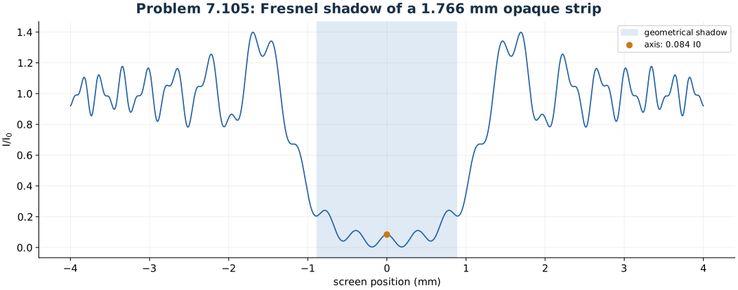
Numerical Fresnel propagation behind the specified opaque strip shows the weak central irradiance and oscillatory lit-side fringes.