Collimation, Lens Alignment, and Focus

These methods separate four easily confused errors: beam divergence, lens decenter, lens tilt, and longitudinal defocus. Correct them in that order; a tilted lens should not be used to hide a decenter error.

Method 3: expand and spatially filter a beam

For a Keplerian telescope with positive focal lengths \(f_1\) and \(f_2\), place the lenses approximately \(f_1+f_2\) apart. The beam diameter magnification and ideal divergence reduction are

(1)\[M=\left|\frac{f_2}{f_1}\right|, \qquad D_{\rm out}=M D_{\rm in}, \qquad \Theta_{\rm out}\simeq\frac{\Theta_{\rm in}}{M}.\]

A pinhole at the shared focus removes high-spatial-frequency contamination. Its starting diameter should exceed the diffraction-limited Airy diameter

(2)\[d_{\rm Airy}=2.44\frac{\lambda f_1}{D_{\rm in}}.\]

Worked example. With \(f_1=25\ \mathrm{mm}\), \(f_2=100\ \mathrm{mm}\), \(D_{\rm in}=1.0\ \mathrm{mm}\), and \(\lambda=532\ \mathrm{nm}\), \(M=4\), the lens spacing starts at 125 mm, and \(D_{\rm out}=4.0\ \mathrm{mm}\). The Airy diameter is 32.5 micrometres, so a 50 micrometre pinhole is a practical initial choice.

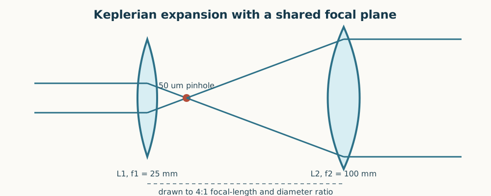
Figure 1. Center the first lens, maximize pinhole transmission in \(x,y,z\), then add the second lens and adjust only its axial location for collimation.

Method 4: test collimation with a shear plate

A shear plate overlaps two laterally displaced copies of the wavefront. For a paraxial spherical wavefront \(W(x)=x^2/(2R)\) and shear \(s\),

(3)\[\Delta W=W(x+s)-W(x)=\frac{s}{R}x+\frac{s^2}{2R}.\]

The \(x\)-dependent term tilts the wedge’s carrier fringes. A collimated beam has \(R\rightarrow\infty\), so that added tilt vanishes. Curved fringes indicate aberration or an off-axis/wrongly oriented lens, not merely simple defocus.

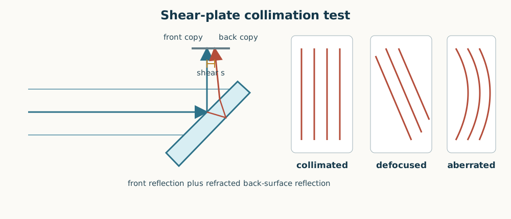
Figure 2. Use the manufacturer’s reference line to interpret sign. Make a small known axial motion first and observe which fringe rotation represents convergence and which represents divergence.

When a shear plate is unavailable, pass a broad beam through two holes separated by \(s\) and measure the spot separation at planes separated by \(L\):

(4)\[\alpha\simeq\frac{s_2-s_1}{L}, \qquad R\simeq\frac{s_1}{\alpha}.\]

For 3.00 mm initial separation increasing to 3.15 mm after 1.00 m, \(\alpha=0.150\ \mathrm{mrad}\) and \(R\simeq20\ \mathrm{m}\). This method is less sensitive than a shear plate but gives a numerical residual.

Method 5: center and square a single lens

First define the axis using two approximately 1 mm irises. Insert one lens, translate it in \(x,y\) until the transmitted focus remains on the axis, then remove tilt using the surface back-reflection. For a narrow collimated ray and thin lens, decenter \(\delta\) produces

(5)\[\theta_{\rm out}\simeq\frac{\delta}{f}, \qquad x(f)\simeq\delta.\]

A 0.20 mm decenter of a 50 mm lens therefore produces a 4.0 mrad ray-angle error and moves the focal spot about 0.20 mm.

For a return screen a distance \(L_r\) from the surface, surface tilt \(\tau\) moves the reflected spot by

(6)\[\Delta x_r\simeq2L_r\tau.\]

Thus a 1.0 mm return error at \(L_r=0.50\ \mathrm{m}\) means \(\tau\simeq1.0\ \mathrm{mrad}\). Center by translation, square by tilt, and iterate because the controls are not perfectly independent.

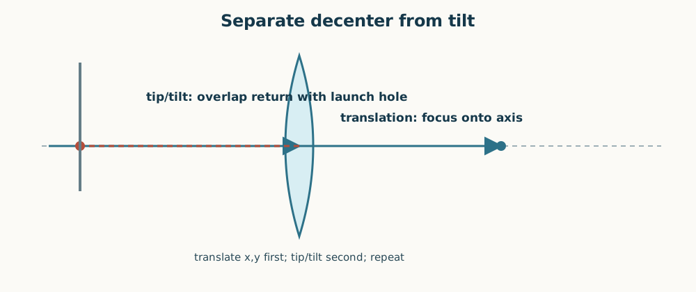
Figure 3. The transmitted beam diagnoses centering; the retroreflected spot diagnoses surface normal. Insert and align one lens at a time.

Method 6: autocollimate a surface

An autocollimator projects a reticle through a collimating objective and images its reflection. If its objective focal length is \(f_a\), a surface tilt \(\tau\) creates image displacement

(7)\[\Delta x\simeq2f_a\tau, \qquad \tau\simeq\frac{\Delta x}{2f_a}.\]

For \(f_a=200\ \mathrm{mm}\) and \(\Delta x=0.10\ \mathrm{mm}\), the surface tilt is 0.25 mrad. Focus the instrument on each surface in turn; use reticle centering for lateral placement and reflected-reticle coincidence for tilt.

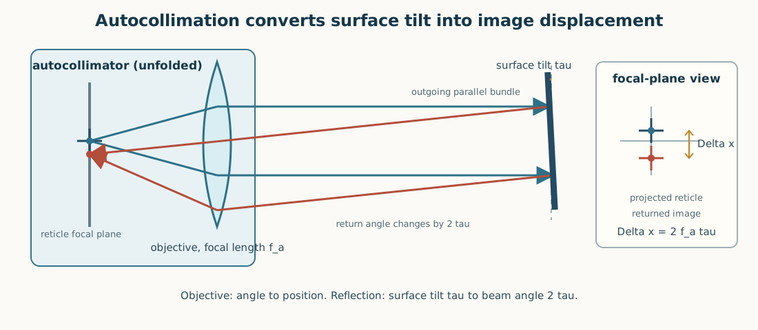
Figure 4. In this unfolded ray diagram, the objective converts a reticle point at its focal plane into a parallel bundle. Surface tilt \(\tau\) changes the return angle by \(2\tau\); the same objective then focuses the return at \(\Delta x\simeq2f_a\tau\). A stable instrument mount is part of the reference and must not be adjusted between elements.

Method 7: locate a focal plane and an objective BFP

For a distant object at distance \(u\), the thin-lens image distance is

(8)\[v=\frac{fu}{u-f}, \qquad v-f=\frac{f^2}{u-f}.\]

With \(f=100\ \mathrm{mm}\) and \(u=5.0\ \mathrm{m}\), the screen focuses at 102.04 mm, not exactly 100 mm. A more distant target reduces that finite-conjugate error. For a short-focus lens, scan a low-power expanded beam across a matte target: the smallest illuminated patch, hence largest observed speckle grains, marks focus.

For an objective back focal plane (BFP), translate the input focusing lens until the output from the objective is collimated. A small axial BFP error \(\Delta z\) gives approximate residual wavefront curvature

(9)\[\frac{1}{R}\simeq\frac{\Delta z}{f_{\rm obj}^2}.\]

For \(f_{\rm obj}=10\ \mathrm{mm}\) and \(\Delta z=10\ \mu\mathrm{m}\), \(R\simeq10\ \mathrm{m}\). Check it on an enclosed distant target or with a shear plate; do not send an open beam across the room.

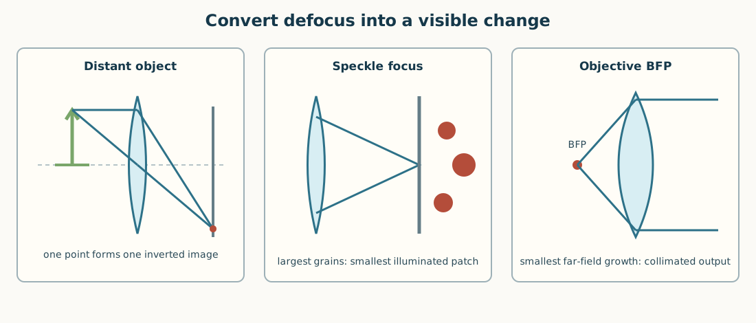
Figure 5. Each method converts longitudinal defocus into an observable: image sharpness, speckle size, or far-field beam growth.